 |
Lecture notes in Transportation Systems Engineering
December 10, 2010


| k | v |
| 171 | 5 |
| 129 | 15 |
| 20 | 40 |
| 70 | 25 |
| x(k) | y(v) | ( |
( |
( |
(
|
| 171 | 5 | 73.5 | -16.3 | -1198.1 | 5402.3 |
| 129 | 15 | 31.5 | -6.3 | -198.5 | 992.3 |
| 20 | 40 | -77.5 | 18.7 | -1449.3 | 6006.3 |
| 70 | 25 | -27.5 | 3.7 | -101.8 | 756.3 |
| 390 | 85 | -2947.7 | 13157.2 |
![\begin{displaymath}
v = v_f{[1-{{\left(\frac{k}{k_j}\right)}^n}]}
\end{displaymath}](img58.png) |
(13) |
| (14) |

| (17) |
| (18) |
| (19) |
| (20) |
| (21) |
| (22) |
| (23) |
 |
(24) |
![\begin{displaymath}
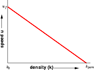
v = v_f -\left[\frac{v_f}{k_j}\right].k
\end{displaymath}](img2.png)
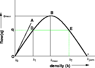
![\begin{displaymath}
q = v_f.k -\left [{\frac{v_f}{k_j}}\right] k^2
\end{displaymath}](img12.png)
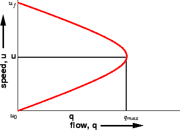
![\begin{displaymath}
q = k_j.v -\left[{\frac{k_j}{v_f}}\right] v^2
\end{displaymath}](img14.png)


