Non-Liner Programming
Lecture notes in Transportation Systems Engineering
4 August 2009
Optimization is the act of obtaining the best result under given circumstances.
It is the process of finding the condtions that give maximum or minimum value of a function.
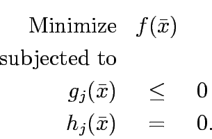
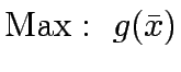
The general form of the optimization problem will be to find  that
that
where is the decision variable.
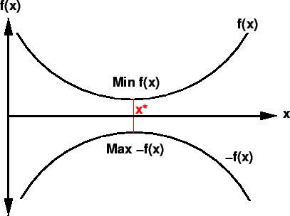
Figure 1 shows the concept of optimization which is to find the minimum or maximum of a function.
Since Minimizing  is same as maximizing
  we shall follow the former notation.
The optimum solution is indicated by
we shall follow the former notation.
The optimum solution is indicated by 
Figure 1:
The concept of optimisation
 |
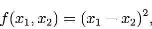
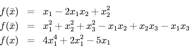
Determin the convexity of the following function:
Determin the convexity of the following functions:
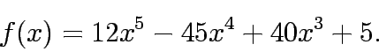
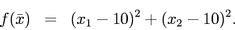
Solve the function and iterpret the results(s):
Solve the following functions and iterpret the results(s):
Solve the function and iterpret the results(s):
Solve the following functions and iterpret the results(s):
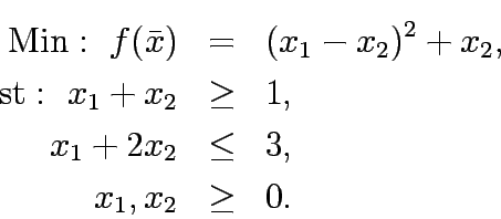
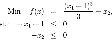
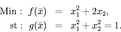
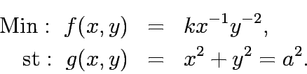
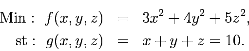
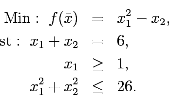
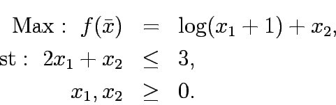
Solve the following constrained program:
Solve the following constrained program:
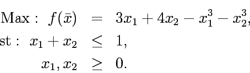
Solve the following constrained program:
Solve the following constrained program:
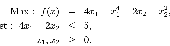
Solve the following constrained program:
Solve the following constrained program:
Solve the following unconstrained one dimentional problem:
Solve the following unconstrained one dimentional problems
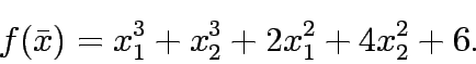
Solve the following unconstrained multi-variable problem:
Solve the following unconstrained multi-variable problems:
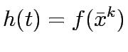
It is type of sequential approximation algorithm.
This is applicable when the objective function is non liner and the constraints are all liner.
It uses a linear approximation of the objetive function and solve by any classical linear programming algorithm.
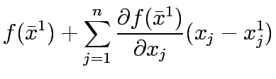
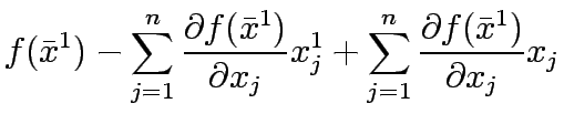
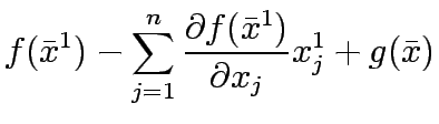
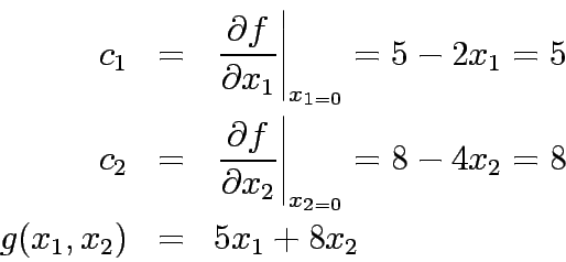
Given a feasible trail solution (
 ), then the linear
approximation used for the objective function is the first order Taylor series
expansion of
), then the linear
approximation used for the objective function is the first order Taylor series
expansion of  around
. Thus
around
. Thus
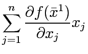
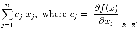
Since the first and second term of is constant, optimzing is same as optimizing  .
Therefore, the equivalent linear form of is , that is,
.
Therefore, the equivalent linear form of is , that is,
- Set
 =0, find initital solution
- Set
 compute
- Find optimum solution
 for the following LP
- For the variable
 set
set
- Find
 that maximizes
  in the interval
  and compute the next point by
![$\displaystyle \bar{x}^k=\bar{x}^{k-1}+t^*\left[\bar{x}^k_{LP} - \bar{x}^{k-1} \right]$](img53.gif) |
|
|
(6) |
- If the error
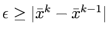 go to step 2, else STOP.
Note that in step 1 use LP to get a feasible initital solution.
Also in step 5 use any one dimentional search (either numerical or classical) to maximize the function .
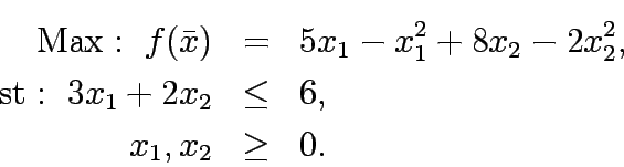
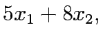
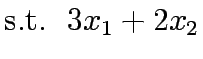
Solve the following program by frank-wolfe alogorithm:
| k |
 |
 |
|
x(t) |
h(t) |
|
 |
| 0 |
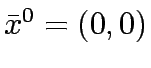
0, 0 |
5, 8 |
0, 3 |
0, 3t |
24t-18t |
2/3 |
0, 2 |
Solve the following program by frank-wolfe alogorithm:
Solve the following program by frank-wolfe alogorithm:
Solve the following program by frank-wolfe alogorithm:
Solve the following program by inner penalty function method:
Solve the following program by exterior penalty function method:
- 1
Mohan c Joshi and Kannan M Moudgalya.
Optimization: Theory and practice.
Narosa Publishing House, New Delhi, India, 2004.
- 2
K. Deb.
Optimization for engineering design: Algorithms and Examples.
Prentice Hall, India, 1998.
- 3
F S Hillier and G J Lieberman.
Introduction to operations research.
McGraw Hill, Inc., 2001.
- 4
Singiresu S Rao.
Engineering optimization: Theory and practice.
New Age International, New Delhi, India, 1996.
- 5
A Ravindran, D T Philips, and J J Solberg.
Operations research: Principles and practice.
John Wiley and Sons, 1987.
- 6
H A Taha.
Operations research: An introduction.
Prentice-Hall, India, 1997.
Prof. Tom V. Mathew
2009-08-04
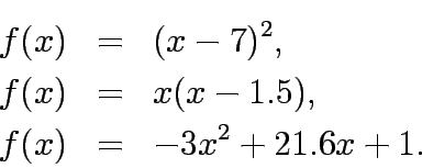
![\begin{eqnarray*}
\mathrm{Min: } f(x)&=&x(x-1.5), [0-1];\\
\mathrm{Min: } f(x...
... && [0-3];\\
\mathrm{Max: } f(x)&=&-3x^2+21.6x+1, [0-25].
\end{eqnarray*}](img19.gif)


![$\displaystyle \bar{x}^k=\bar{x}^{k-1}+t\left[\bar{x}^k_{LP} - \bar{x}^{k-1} \right]$](img49.gif)

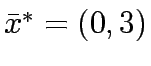
![$\bar{x}^k=(0,0)+t[(0,3)-(0,0)]=(0,3t)$](img66.gif)

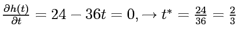
![$x_k=(0,[3\times\frac{2}{3}])=(0,2)$](img69.gif)