Transportation networks

Lecture notes in Transportation Systems Engineering

4 August 2009

1 Singel O-D netowrks: Link flows

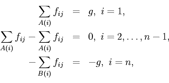
The conservation equation for a network can be written as:

$$\begin{eqnarray*} \sum_{A(i)} f_{ij} &=& g,  i=1,\\ \sum_{A(i)} f_{ij} - \sum_... ...&=& 0,  i=2,\dots,n-1,\\ -\sum_{B(i)} f_{ij} &=& -g,  i=n,\\ \end{eqnarray*}$$

where, $g$ denote the flow value, and $f_{ij}$ is the flow on link i,j.

The net flow across any cut-set $(X,\bar{X})$ separating the origin and destination is equal to the flow value.

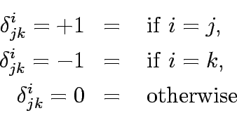
The conservation equation can be conveniently represented in a matrix form. The node-link incidence matrix in an $n\times l$ matrix ${\bf E}$ where the rows corresponds to nodes ($i$)and the column corresponds to links $(j,k)$ and each cell denoted by $\delta^i_{jk}$ defined as:

$$\begin{eqnarray*} \delta^i_{jk}=+1 &=& \mathrm{if}  i=j,\\ \delta^i_{jk}=-1 &=& \mathrm{if}  i=k,\\ \delta^i_{jk}=0 &=& \mathrm{otherwise}\\ \end{eqnarray*}$$

For example ...

$$\begin{eqnarray*} {\bf E}=\left[ \begin{array}{cccccc} 1 & 1 & 0 & 0 & 0 & 0 ... ...-1 & 0 & 1 & 1 \\ 0 & 0 & 0 &-1 & 0 &-1 \\ \end{array}\right] \end{eqnarray*}$$

The flow conservation equations () can now be written as:

$${\bf Ef=g}$$ (1)

where ${\bf f}$ is the vector of link flows, ${\bf g}$ is the O-D vector.

2 Minimal spanning tree

In a connected weighted graph, all spanning trees have n-1 edges and will have minimum or maximum sum of the weights. Tow algorithms are proposed: Prims algorithma dn Kruskal's algorithm. `

2.1 Prims algorithm

Prims algorithm grows a spanning tree from a given vertex of a connected weighted graph G, iteratively adding the cheapest edge from a vertex already reached to a vertex not yet reached, finishing when all the vertices of G have been reached. Break tie arbitrarily. Input: A weighted, connected graph G(N,L) Initilisation: T(G)=$\Phi$ Iteration: Add cheapest edge that incorporate a new vertex

2.1.0.1 Example

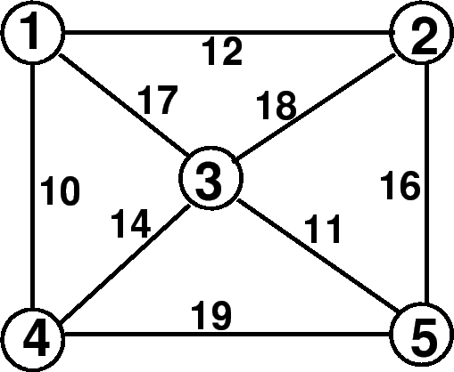
Find the minimum spanning tree of the network given in figure 1

Figure 1: Example netowrk for minimum spanning tree problem 1

2.1.0.2 Solution

1. Start with node 1, N={1}, T={$\Phi$}
2. Node 1 can be connected by nodes 2, 3, and 4, having weights 12, 17, and 10
3. Minimim weight is 10, for node 4. So N={1,4}, T={(1,4)}
4. Node 1 can be connected by nodes 2 and 3, having weights 12 and 17
5. Node 4 can be connected by nodes 3 and 5, having weights 14 and 19
6. Minimim weight is 12, for node 2. So N={1,4,2}, T={(1,4),(1,2)}
7. Node 1 can be connected by node 3, having weight 17
8. Node 4 can be connected by nodes 3 and 5, having weights 14 and 19
9. Node 2 can be connected by nodes 3 and 5, having weights 18 and 16
10. Minimim weight is 14, for node 3. So N={1,4,2,3}, T={(1,4),(1,2),(3,4)}
11. Node 1 can be connected by no nodes without loop
12. Node 4 can be connected by node 5, having weight 19
13. Node 2 can be connected by node 5, having weight 16
14. Node 3 can be connected by node 5, having weight 11
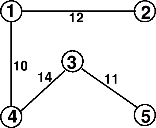
15. Minimim weight is 11, for node 3. So N={1,4,2,3}, T={(1,4),(1,2),(3,4),(3,5)} W=49.

Figure 2: Solution for the example netowrk for minimum spanning tree problem 1

2.2 Kruskal's algorithm

The main concept of this algorithm is to maintain an acyclic spanning sub-graph H, enlargin it by edges with low weight to form a spanning tree. Consider edges in non-descending order of weight, breaking ties arbitrarily.

Input: A weighted connected graph G(N,L) Initilization: Set T=$\Phi$ a sub-graph of G Iteration: If the next cheapest edge joins two components of T, then include it, otherwise, discard it. Terminate when T is connected.

2.2.0.1 Example

Find the minimum spanning tree of the network given in figure 1

2.2.0.2 Solution

1. Sort the links in the descending order of weights reslts in
2. 19 (4,5); 18 (2,3); 17 (1,3); 16 (2,5); 14 (3,4); 12 (1,2); 11 (3,5); and 10 (1,4)
3. T=(1,4) W=10
4. T=(1,4),(3,5) W=10+11
5. T=(1,4),(3,5),(1,2), W=10+11+12
6. T=(1,4),(3,5),(1,2),(3,4), W=10+11+12+14=47

3 Dijkstra's shortest path algorithms

Input: A graph with nonnegative edge weights and a starting vertex $u$. The weight of $xy$ is $w(xy)$; let $w(xy)=\infty$ if $xy$ is not an edge. Initilization: Set $S={u};  t(u)=0;  t(z)=W(uz)$ for $z\neq u$ Iteration: Select a vertex $v$ outside $S$ such that $t(v)=min_{z\notin S} t(z)$ Add $v$ to $S$. Explore edges from $v$ to update tentative distances: for each edge $vZ$ with $x\notin S$, update $t(z)$ to minimize $\{t(z), t(v)+w(vz)\}$ Iteration continues until $S=V(G)$ or until $t(z)=infty$ for every $z\notin S$. At the end, set $d(u,v)=t(v) \forall v$

3.0.0.1 Solution

Table 1: Solution to the shortest path algorithm

$\{S\}$	$v$	$vz$	$t(v)+w(vz)$	$t^*(z)$	$z^*$	$s^*$
u	u	ua	0+1=1	1	a	ua
		ub	0+3=3
ua	u	ub	0+3=3	3	b	uab
	a	ad	1+5=6
		ac	1+4=4
uab	a	ad	1+5=6
		ac	1+4=5	5	c	uabc
	b	bd	3+4=7
		bc	3+5=8
uabc	a	ad		6	d	uabcd
uabcd						uabcdv

Bibliography

1 Renfrey B Potts and Robert M Oliver. Flows in transportation networks. Academic Press, New York, 1972.

2 Douglas B West. Introduction to graph theory. Pearson education Asia, New Delhi, India, 2001.