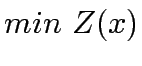
Transport Network Design
Lecture notes in Transportation Systems Engineering
4 August 2009
This document discusses the aspects of network design.
The reader assumed to be familiar with the basics of various types of traffic assignment
techniques especailly user equilibrium and system optimum including the mathematical formulation and
solution approaches.
Then the concept of bilevel
programming and few examples will be presented.
Finally one such example, namely
the network capacity expansion will be formulated as a bilevel optimization
problem and will be illustrated using a numerical example.
Transportation network design in a broad sense deeds with the
configuration of network to achieve specified objectives.There are two
variations to the problem, the continuous network design and the discrete
network design. Examples of the form include
- a
The determination of road width.
- b
The calculation of signal timings.
- c
The setting of road user charges.
Although this document covers the continous network design in detailed, basis
underlinig principles are some form the discrete case.
Conventional network design has been concerned with minimization of total
system cost.However, this may be unrealistic in the sense that how the user
will respond to the proposed changes is not considered.
Therefore, currently the network designis thought of as supply demand problem
or leader-follower game.The system designer leads, taking into account how the
user follow.
The core of all network design problems is how a user chooses his route of
travel.
The class of traffic assignment problem tries to model these behaviour.
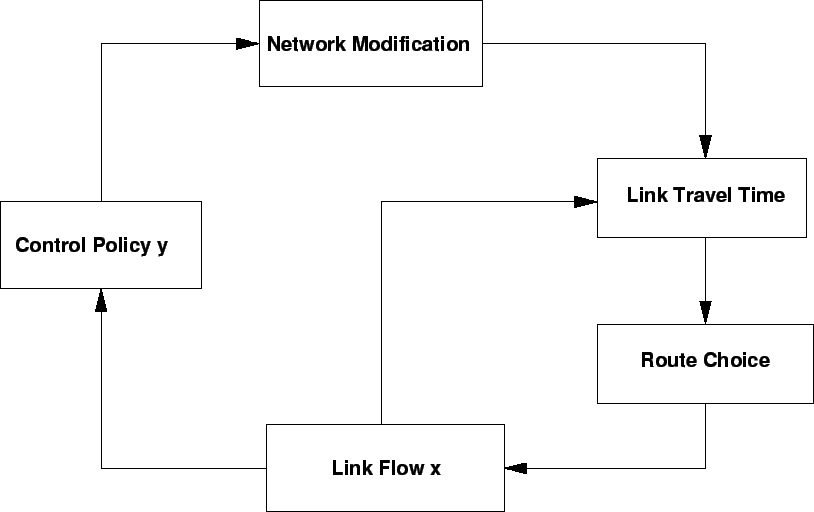
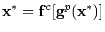
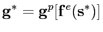
The bilevel programming (BLP) problem is a special case of multilevel
programming problems with a two level structure. The problem can be expressed
as follows: the transport planner, wishes to determine an optimal policy as a
function of his or control variables (y) and the users response to these
controls, where users response generally takes the form of a network flow (x).
The transport planner then seeks to minimise a function of both y and
x, where some constraints may be imposed upony as well as the fact
that x should be a user equilibrium flow, parameterised by the control
vector,y. There exists many problems in transportation that can be
formulated as bilevel programming problem.They include network capacity
expansion, network level signal setting and optimum toll pricing. They are
discussed briefly here:
The network capacity expansion problem is to determine capacity enhancements of
existing facilities of a transportation network which are, in some sense,
optimal. Network design models concerned with adding indivisible facilities
(modeled as integer variables) are said to be discrete, whereas those
dealing with divisible capacity enhancements (modeled as continuous variables)
are said to be continuous.
Thus network expansion problem is a continuous network design problem,which
determines the set of link capacity expansions and the corresponding
equilibrium flows for which measures of performance index for network is
optimal. A bilevel programming technique can be used to formulate this
equilibrium network design problem. At the upper level problem, the system
performance index is defined as the sum of total travel times and investment
costs of link capacity expansions. At the lower level problem, the user
equilibrium flow is determined by Wardrop's first principle and can be
formulated as an equivalent minimization problem. The most well-studied
equilibrium network design problem is user equilibrium network design with
fixed transportation demand.
For a road network with flow responsive signal control and fixed
origin-destination travel demands. Combined traffic assignment and signal
control problem tries to allocate the demand matrix to the network subject to
user equilibrium assumption and computes the optimal signal control parameter
from the generated link flows.Consider f and g, which denote
respectively, a vector of link flows and a vector of signal settings for the
network; assuming that the signal plan structure is given (specified by number,
type, and sequence of phases), signal settings may consist of cycle length's,
green splits, and offsets.Traffic equilibrium, is a set of link
flows satisfying satisfying Wardrop's first principle.
is a set of link
flows satisfying satisfying Wardrop's first principle.
The equilibrium traffic signal setting is a pair
 such that
  is a traffic equilibrium when signals are set at
 .
.
 |
(1) |
where  is the signal settings corresponding to
under specified control policy P;
is the signal settings corresponding to
under specified control policy P;
 |
(2) |
If there exists a pair
 , then link flows
and signal settings are
, then link flows
and signal settings are
In general,traffic flow and queue size on a road network depend on road toll
pattern and also traffic control. An efficient pricing scheme should therefore
take into account the effects of the altered network flow pattern and queueing
due to road pricing to achieve a global optimal solution. This requires
development of an efficient procedure for calculating optimal toll patterns in
general road networks while anticipating driver response in terms of route
choice. The procedure should be able to estimate queueing delay and queue
length, both of which are critical in queue management in congested urban road
networks. Optimum toll pricing problem can be formulated as a bilevel
programming in general road networks. The users route choice behaviour under
condition of queing and congestion in a road network for any given toll pattern
can be represented by the mathematical programming model.Global evaluation of
likely effects of road pricing thud becomes possible.The model can be
formulated to find an optimal set of link tolls such that a particular system
performance criterion is optimized.A meaningful objective is to optimize is to
minimize the total network cost or to maximize total revenue raised from toll
charges. In this kind of problem,it is assumed that for any given toll
pattern,u,there is a unique equilibrium flow
distribution,x,obtained from the lower-level problem. x is also
called the response or reaction function.
An efficient toll pattern,u, will greatly depend on how to evaluate the
reaction function x, or in other words,how to predict route changes of
users in response to alternative toll charges.
This interaction game can be represented as the following bi-level programming
problem:
Lower Level:
where  is the signal settingd corresponding to
  under specified control
policy P;
under specified control
policy P;
If there exists such a pair  , then link flows and signal settings are
There can be be three types of formulation on upper level,
one is total network travel cost  , the sum of travel times and queueing delays experienced by
all vehicles:
, the sum of travel times and queueing delays experienced by
all vehicles:
The total revenue, denoted as  , arising from toll charges can be expressed as:
A third objective function can be to maximize the ratio, denoted as
 , of the total revenue to total cost :
where  is travel cost
  is exit flows and
  are the queueing
delay.
are the queueing
delay.
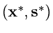
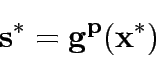
Consider a road network and suppose that origin destination travel demand is fixed and known. Let x and y denote respectively vector of link flows and a vector of network expansion policy. A Budget control policy, denoted by B is in general any rule or procedure that can be used to determine the components of 'y' when 'x' is known. The network design problem consists of finding a pair
 ,such that
  is at traffic equilibrium when capacity is
  .
.
where is the capacity improvement corresponding to a under specified Budget B and  is the function that gives the vector of link flows.
where  is a function that given optimal capacity expansion vector for a given
  .
If there exists such a pair (, ) then link flows and capacity improvement are mutually consistent or in equilibrium , in the sense that users choice when controls are at yield link flows equal to those from which arises under budget constraint B.In other words
.
If there exists such a pair (, ) then link flows and capacity improvement are mutually consistent or in equilibrium , in the sense that users choice when controls are at yield link flows equal to those from which arises under budget constraint B.In other words
or equivalently
Figure 1:
Bilevel
 |
The following notation has been used for CNDP formulation:
Let A be the set of links in the network,  the set of OD pairs,
q the vector of fixed OD pair demands,q =
the set of OD pairs,
q the vector of fixed OD pair demands,q =  ,
K the set of paths between OD pair
,
K the set of paths between OD pair  , f the vector of path flows between OD pair r,s on path k which means f = [
 ],
x the vector of link flows, x =
],
x the vector of link flows, x =  , y the vector of link capacity expansion,
y =
, y the vector of link capacity expansion,
y =  , B the allocated budget for expansion,
  travel time on link a,
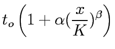
 is the coefficient of link expansion vector y,, flow on path k connecting O-D pair r-s,
 trip rate between r and s.
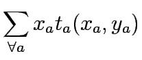
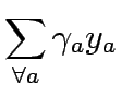
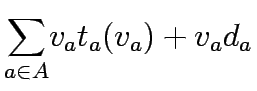
Upper Level
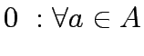
subject to
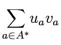
Lower Level
subject t
 equilibrium flows in link a, travel time on link a,
  link capacity expansions in link a,
  , flow on path k connecting O-D pair r-s, trip rate between r and s.
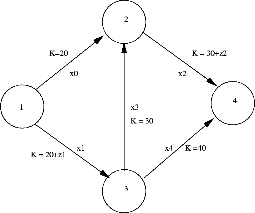
To illustrate how the bilevel problem of network capacity expansion works an example network
was considered.This network had four nodes and five links.Two links were considered for improvement.
The figure shows the network.
, flow on path k connecting O-D pair r-s, trip rate between r and s.
To illustrate how the bilevel problem of network capacity expansion works an example network
was considered.This network had four nodes and five links.Two links were considered for improvement.
The figure shows the network.
Figure 2:
Bilevel example problem
 |
| From |
To |
 |
 |
length(Km) |
Capacity(K) |
Speed(Km/hr) |
| 1 |
2 |
0.15 |
4.0 |
1.0 |
20.0 |
60.0 |
| 1 |
3 |
0.15 |
4.0 |
1.0 |
20.0 |
60.0 |
| 2 |
4 |
0.15 |
4.0 |
1.0 |
30.0 |
60.0 |
| 3 |
2 |
0.15 |
4.0 |
1.0 |
30.0 |
60.0 |
| 3 |
4 |
0.15 |
4.0 |
1.0 |
40.0 |
60.0 |
| no. |
x0* |
x1* |
x2* |
x3* |
x4* |
UE |
TSTT |
z1* |
z2* |
SO |
| 1 |
42.5 |
38.71 |
52.87 |
10.37 |
79.09 |
317.39 |
692.8 |
5.36 |
4.64 |
609.41 |
| 2 |
38.78 |
42.27 |
56.05 |
17.27 |
75.65 |
296.85 |
564.23 |
5.79 |
4.21 |
564 |
| 3 |
38.61 |
42.44 |
55.67 |
17.06 |
76.02 |
296.73 |
564.48 |
5.95 |
4.05 |
564.45 |
| 4 |
38.45 |
42.56 |
55.58 |
17.13 |
76.07 |
296.53 |
563.5 |
6.02 |
3.98 |
563.5 |
| 5 |
38.51 |
42.53 |
55.48 |
16.97 |
76.21 |
296.68 |
564.61 |
6.04 |
3.96 |
564.61 |
| 6 |
38.5 |
42.53 |
55.46 |
16.96 |
76.22 |
296.66 |
564.6 |
6.04 |
3.96 |
564.6 |
The initial link expansion vector is taken as 0. User equilibrium is performed to get the required link flows. Now these
flows are input to upper level from where we get a new set of link expansion vectors which minimizes the system
travel time.This iteration is repeated until the total sytem travel time from lower level and
upper level converges.
- 1
Yosef Sheffi.
Urban transportation networks: Equilibrium analysis with
mathematical programming methods.
New Jersey, 1984.
- 2
R Thomas.
Traffic Assignment Techniques.
Avebury Technical publication,England, 1991.
Prof. Tom V. Mathew
2009-08-04


![$\displaystyle x^e [y^P (x^\ast )] \mid constant y$](img42.gif)
![$\displaystyle y^P [x^e(y^\ast )] \mid constant x$](img43.gif)