Introduction to Travel Demand Modeling

Lecture notes in Transportation Systems Engineering

July 28, 2011

Overview

This chapter provides an introduction to travel demand modeling, the most important aspect of transportation planning. First we will discuss about what is modeling, the concept of transport demand and supply, the concept of equilibrium, and the traditional four step demand modeling. We may also point to advance trends in demand modeling.

Transport modeling

Modeling is an important part of any large scale decision making process in any system. There are large number of factors that affect the performance of the system. It is not possible for the human brain to keep track of all the player in system and their interactions and interrelationships. Therefore we resort to models which are some simplified, at the same time complex enough to reproduce key relationships of the reality. Modeling could be either physical, symbolic, or mathematical In physical model one would make physical representation of the reality. For example, model aircrafts used in wind tunnel is an example of physical models. In symbolic model, with the complex relations could be represented with the help of symbols. Drawing time-space diagram of vehicle movement is a good example of symbolic models. Mathematical model is the most common type when with the help of variables, parameters, and equations one could represent highly complex relations. Newton's equations of motion or Einstein's equation $E={m}{c}^2$, can be considered as examples of mathematical model. No model is a perfect representation of the reality. The important objective is that models seek to isolate key relationships, and not to replicate the entire structure. Transport modeling is the study of the behavior of individuals in making decisions regarding the provision and use of transport. Therefore, unlike other engineering models, transport modeling tools have evolved from many disciplines like economics, psychology, geography, sociology, and statistics.

Transport demand and supply

The concept of demand and supply are fundamental to economic theory and is widely applied in the field to transport economics. In the area of travel demand and the associated supply of transport infrastructure, the notions of demand and supply could be applied. However, we must be aware of the fact that the transport demand is a derived demand, and not a need in itself. That is, people travel not for the sake of travel, but to practice in activities in different locations

The concept of equilibrium is central to the supply-demand analysis. It is a normal practice to plot the supply and demand curve as a function of cost and the intersection is then plotted in the equilibrium point as shown in Figure 1

Figure 1: Demand supply equilibrium

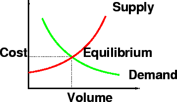The demand for travel T is a function of cost C is easy to conceive. The classical approach defines the supply function as giving the quantity T which would be produced, given a market price C. Since transport demand is a derived demand, and the benefit of transportation on the non-monetary terms(time in particular), the supply function takes the form in which C is the unit cost associated with meeting a demand T. Thus, the supply function encapsulates response of the transport system to a given level of demand. In other words, supply function will answer the question what will be the level of service of the system, if the estimated demand is loaded to the system. The most common supply function is the link travel time function which relates the link volume and travel time.

Travel demand modeling

Travel demand modeling aims to establish the spatial distribution of travel explicitly by means of an appropriate system of zones. Modeling of demand thus implies a procedure for predicting what travel decisions people would like to make given the generalized travel cost of each alternatives. The base decisions include the choice of destination, the choice of the mode, and the choice of the route. Although various modeling approaches are adopted, we will discuss only the classical transport model popularly known as four-stage model(FSM).

The general form of the four stage model is given in Figure 2.

Figure 2: General form of the four stage modeling

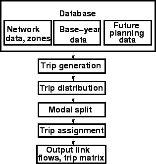The classic model is presented as a sequence of four sub models: trip generation, trip distribution, modal split, trip assignment. The models starts with defining the study area and dividing them into a number of zones and considering all the transport network in the system. The database also include the current (base year) levels of population, economic activity like employment, shopping space, educational, and leisure facilities of each zone. Then the trip generation model is evolved which uses the above data to estimate the total number of trips generated and attracted by each zone. The next step is the allocation of these trips from each zone to various other destination zones in the study area using trip distribution models. The output of the above model is a trip matrix which denote the trips from each zone to every other zones. In the succeeding step the trips are allocated to different modes based on the modal attributes using the modal split models. This is essentially slicing the trip matrix for various modes generated to a mode specific trip matrix. Finally, each trip matrix is assigned to the route network of that particular mode using the trip assignment models. The step will give the loading on each link of the network.

The classical model would also be viewed as answering a series of questions (decisions) namely how many trips are generated, where they are going, on what mode they are going, and finally which route they are adopting. The current approach is to model these decisions using discrete choice theory, which allows the lower level choices to be made conditional on higher choices. For example, route choice is conditional on the mode choice. This hierarchical choices of trip is shown in Figure 3

Figure 3: Demand supply equilibrium

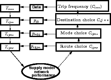The highest level to find all the trips $T_{i}$ originating from a zone is calculated based on the data and aggregate cost term $C_{i}$***. Based on the aggregate travel cost $C_{ij}$** from zone $i$ to the destination zone $j$, the probability $p_{m\mid{ij}}$ of trips going to zone $j$ is computed and subsequently the trips $T_{ij}$** from zone $i$ to zone $j$ by all modes and all routes are computed. Next, the mode choice model compute the probability $p_{m\mid{ij}}$ of choosing mode $m$ based on the travel cost $C_{jm}$* from zone $i$ to zone $j$, by mode $m$ is determined. Similarly, the route choice gives the trips $T_{ijmr}$ from zone $i$ to zone $j$ by mode $m$ through route $r$ can be computed. Finally the travel demand is loaded to the supply model, as stated earlier, will produce a performance level. The purpose of the network is usually measured in travel time which could be converted to travel cost. Although not practiced ideally, one could feed this back into the higher levels to achieve real equilibrium of the supply and demand.

Summary

In a nutshell, travel demand modeling aims at explaining where the trips come from and where they go,and what modes and which routes are used. It provides a zone wise analysis of the trips followed by distribution of the trips, split the trips mode wise based on the choice of the travelers and finally assigns the trips to the network. This process helps to understand the effects of future developments in the transport networks on the trips as well as the influence of the choices of the public on the flows in the network.

Problems

1. Link travel time function relates travel time and
   1. link volume
   2. link cost
   3. level of service
   4. none of the above
2. What is the first stage of four-stage travel demand modeling?
   1. Trip generation
   2. Trip distribution
   3. Modal split
   4. Traffic assignment

Solutions

1. Link travel time function relates travel time and
   1. link volume$\surd$
   2. link cost
   3. level of service
   4. none of the above
2. What is the first stage of four-stage travel demand modeling?
   1. Trip distribution
   2. Trip generation$\surd$
   3. Modal split
   4. Traffic assignment

Bibliography