Trip Generation
Lecture notes in Transportation Systems Engineering
August 8, 2011
Trip generation is the first stage of the classical first generation aggregate
demand models.
The trip generation aims at predicting the total number of trips generated and
attracted to each zone of the study area.
In other words this stage answers the questions to ``how many
trips" originate at each zone, from the data on household and
socioeconomic attributes.
In this section basic definitions, factors affecting trip generation, and the
two main modeling approaches; namely growth factor modeling and regression
modeling are discussed.
Some basic definitions are appropriate before we address the classification of
trips in detail.
We will attempt to clarify the meaning of journey, home based trip, non home
based trip, trip production, trip attraction and trip generation.
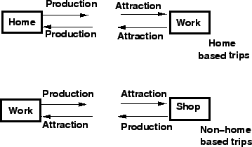
Journey is an out way movement from a point of origin to a point of
destination, where as the word ``trip" denotes an outward and return journey.
If either origin or destination of a trip is the home of the trip maker then
such trips are called home based trips and the rest of the trips are called
non home based trips.
Trip production is defined as all the trips of home based or as the origin of
the non home based trips.
See figure 1
Figure 1:
trip types
 |
Trips can be classified by trip purpose, trip time of the day, and by
person type.
Trip generation models are found to be accurate if separate models are used
based on trip purpose.
The trips can be classified based on the purpose of the journey as trips for
work, trips for education, trips for shopping, trips for recreation and other
trips.
Among these the work and education trips are often referred as mandatory trips
and the rest as discretionary trips.
All the above trips are normally home based trips and constitute about 80 to 85
percent of trips.
The rest of the trips namely non home based trips, being a small proportion are
not normally treated separately.
The second way of classification is based on the time of the day when the trips
are made.
The broad classification is into peak trips and off peak trips.
The third way of classification is based on the type of the individual who
makes the trips.
This is important since the travel behavior is highly influenced by the socio
economic attribute of the traveler and are normally categorized based on the
income level, vehicle ownership and house hold size.
The main factors affecting personal trip production include income, vehicle
ownership, house hold structure and family size.
In addition factors like value of land, residential density and accessibility
are also considered for modeling at zonal levels.
The personal trip attraction, on the other hand, is influenced by factors such
as roofed space available for industrial, commercial and other services.
At the zonal level zonal employment and accessibility are also used.
In trip generation modeling in addition to personal trips, freight trips are
also of interest.
Although the latter comprises about 20 percent of trips, their contribution to
the congestion is significant.
Freight trips are influenced by number of employees, number of sales and area
of commercial firms.
Growth factor modes tries to predict the number of trips produced or attracted
by a house hold or zone as a linear function of explanatory variables.
The models have the following basic equation:
 |
(1) |
where  is the number of future trips in the zone and
  is the number
of current trips in that zone and
is the number
of current trips in that zone and  is a growth factor.
The growth factor depends on the explanatory variable such as population
(P) of the zone , average house hold income (I) , average vehicle ownership
(V).
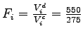
The simplest form of is represented as follows
is a growth factor.
The growth factor depends on the explanatory variable such as population
(P) of the zone , average house hold income (I) , average vehicle ownership
(V).
The simplest form of is represented as follows
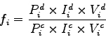 |
(2) |
where the subscript " d" denotes the design year and the subscript "c" denotes
the current year.
Given that a zone has 275 household with car and 275 household without car and
the average trip generation rates for each groups is respectively 5.0 and 2.5
trips per day.
Assuming that in the future, all household will have a car, find the growth
factor and future trips from that zone, assuming that the population and income
remains constant.
Current trip rate
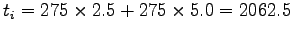 trips / day.
Growth factor
trips / day.
Growth factor
 = 2.0
Therefore, no. of future trips
= 2.0
Therefore, no. of future trips
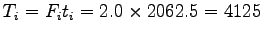 trips / day.
The above example also shows the limitation of growth factor method.
If we think intuitively, the trip rate will remain same in the future.
Therefore the number of trips in the future will be
trips / day.
The above example also shows the limitation of growth factor method.
If we think intuitively, the trip rate will remain same in the future.
Therefore the number of trips in the future will be
 house holds
  5 trips per day = 2750 trips per day .
It may be noted from the above example that the actual trips generated is much lower than the growth factor method.
Therefore growth factor models are normally used in the prediction of external
trips where no other methods are available.
But for internal trips , regression methods are more suitable and will be
discussed in the following section.
The general form of a trip generation model is
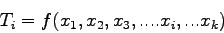 |
(3) |
Where xi's are prediction factor or explanatory variable.
The most common form of trip generation model is a linear function of the form
 |
(4) |
where  's are the coefficient of the regression equation and can be
obtained by doing regression analysis.
The above equations are called multiple linear regression equation, and the
solutions are tedious to obtain manually.
However for the purpose of illustration, an example with one variable is given.
's are the coefficient of the regression equation and can be
obtained by doing regression analysis.
The above equations are called multiple linear regression equation, and the
solutions are tedious to obtain manually.
However for the purpose of illustration, an example with one variable is given.
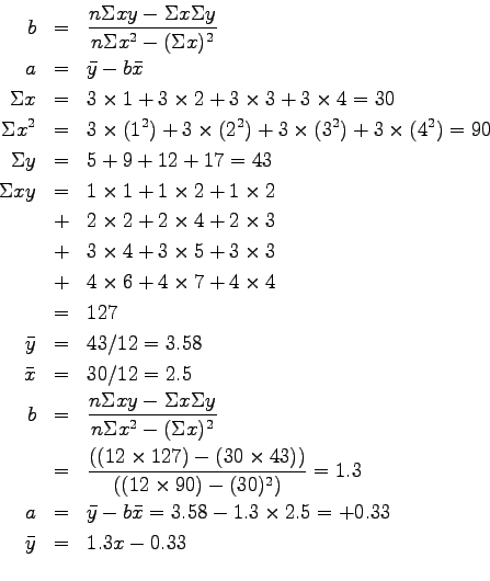
Let the trip rate of a zone is explained by the household size done from the
field survey.
It was found that the household size are 1, 2, 3 and 4.
The trip rates of the corresponding household is as shown in the table below.
Fit a linear equation relating trip rate and household size.
| Household size(x) |
| |
1 |
2 |
3 |
4 |
| Trips |
1 |
2 |
4 |
6 |
| per |
2 |
4 |
5 |
7 |
| day(y) |
2 |
3 |
3 |
4 |
 |
5 |
9 |
12 |
17 |
|
The linear equation will have the form
 where y is the trip rate, and x is the household size, a and b are the
coefficients.
For a best fit, b is given by
where y is the trip rate, and x is the household size, a and b are the
coefficients.
For a best fit, b is given by
Trip generation forms the first step of four-stage travel modeling.
It gives an idea about the total number of trips generated to and
attracted from different zones in the study area.
Growth factor modeling and regression methods can be used to predict
the trips.
They are discussed in detail in this chapter.
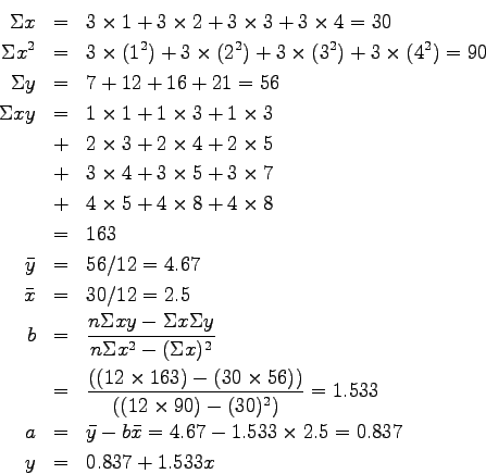
- The trip rate (
 ) and the corresponding household sizes (
 ) from a
sample are shown in table below.
Compute the trip rate if the average household size is 3.25 (Hint: use
regression method).
) from a
sample are shown in table below.
Compute the trip rate if the average household size is 3.25 (Hint: use
regression method).
| |
Householdsize(x) |
| |
1 |
2 |
3 |
4 |
| Trips |
1 |
3 |
4 |
5 |
| per |
3 |
4 |
5 |
8 |
| day(y) |
3 |
5 |
7 |
8 |
Fit the regression equation as below.
When average household size =3.25, number of trips becomes,
 = 5.819
Prof. Tom V. Mathew
2011-08-08