Trip Distribution
Lecture notes in Transportation Systems Engineering
August 10, 2011
The decision to travel for a given purpose is called trip generation.
These generated trips from each zone is then distributed to all other zones
based on the choice of destination.
This is called trip distribution which forms the second stage of travel demand
modeling.
There are a number of methods to distribute trips among destinations; and two
such methods are growth factor model and gravity model.
Growth factor model is a method which respond only to relative growth rates at
origins and destinations and this is suitable for short-term trend
extrapolation.
In gravity model, we start from assumptions about trip making behavior and the
way it is influenced by external factors.
An important aspect of the use of gravity models is their calibration, that is
the task of fixing their parameters so that the base year travel pattern is
well represented by the model.
The trip pattern in a study area can be represented by means of a trip matrix
or origin-destination (O-D)matrix.
This is a two dimensional array of cells where rows and columns represent each
of the zones in the study area.
The notation of the trip matrix is given in figure 1.
Figure 1:
Notation of an origin-destination trip matrix
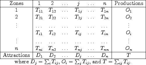 |
The cells of each row  contain the trips originating in that zone which have
as destinations the zones in the corresponding columns.
contain the trips originating in that zone which have
as destinations the zones in the corresponding columns.
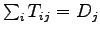
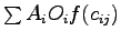
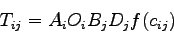
 is the number of trips between origin and destination
  .
.
 is the total number of trips between originating in zone and
  is
the total number of trips attracted to zone .
The sum of the trips in a row should be equal to the total number of trips
emanating from that zone.
The sum of the trips in a column is the number of trips attracted to that zone.
These two constraints can be represented as:
is
the total number of trips attracted to zone .
The sum of the trips in a row should be equal to the total number of trips
emanating from that zone.
The sum of the trips in a column is the number of trips attracted to that zone.
These two constraints can be represented as:

 If reliable information is available to estimate both and , the
model is said to be doubly constrained.
In some cases, there will be information about only one of these constraints,
the model is called singly constrained.
If reliable information is available to estimate both and , the
model is said to be doubly constrained.
In some cases, there will be information about only one of these constraints,
the model is called singly constrained.
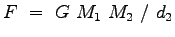
One of the factors that influences trip distribution is the relative travel
cost between two zones.
This cost element may be considered in terms of distance, time or money units.
It is often convenient to use a measure combining all the main attributes
related to the dis-utility of a journey and this is normally referred to as the
generalized cost of travel.
This can be represented as
 |
(1) |
where  is the in-vehicle travel time between and
,
is the in-vehicle travel time between and
,  is the walking time to and from stops,
  is the
waiting time at stops,
is the
waiting time at stops,  is the fare charged to travel between and
,
is the fare charged to travel between and
,  is the parking cost at the destination, and
  is a
parameter representing comfort and convenience, and
is a
parameter representing comfort and convenience, and  ,
,  , .... are the
weights attached to each element of the cost function.
, .... are the
weights attached to each element of the cost function.
If the only information available is about a general growth rate for the whole
of the study area, then we can only assume that it will apply to each cell in
the matrix, that is a uniform growth rate.
The equation can be written as:
 |
(2) |
where  is the uniform growth factor
  is the previous total number of
trips, is the expanded total number of trips.
Advantages are that they are simple to understand, and they are useful for
short-term planning.
Limitation is that the same growth factor is assumed for all zones as well as
attractions.
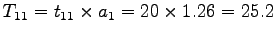
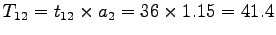
Trips originating from zone 1, 2, and 3 of a study area are 78, 92 and 82
respectively and those terminating at zones 1, 2, and 3 are given as 88, 96 and
78 respectively.
If the growth factor is 1.3 and the base year trip matrix is as given below,
find the expanded origin-constrained growth trip table.
is the previous total number of
trips, is the expanded total number of trips.
Advantages are that they are simple to understand, and they are useful for
short-term planning.
Limitation is that the same growth factor is assumed for all zones as well as
attractions.
Trips originating from zone 1, 2, and 3 of a study area are 78, 92 and 82
respectively and those terminating at zones 1, 2, and 3 are given as 88, 96 and
78 respectively.
If the growth factor is 1.3 and the base year trip matrix is as given below,
find the expanded origin-constrained growth trip table.
| |
1 |
2 |
3 |
 |
| 1 |
20 |
30 |
28 |
78 |
| 2 |
36 |
32 |
24 |
92 |
| 3 |
22 |
34 |
26 |
82 |
 |
88 |
96 |
78 |
252 |
Given growth factor = 1.3,
Therefore, multiplying the growth factor with each of the cells in the matrix
gives the solution as shown below.
| |
1 |
2 |
3 |
|
| 1 |
26 |
39 |
36.4 |
101.4 |
| 2 |
46.8 |
41.6 |
31.2 |
119.6 |
| 3 |
28.6 |
44.2 |
33.8 |
106.2 |
|
101.4 |
124.8 |
101.4 |
327.6 |
When information is available on the growth in the number of trips originating
and terminating in each zone, we know that there will be different growth rates
for trips in and out of each zone and consequently having two sets of growth
factors for each zone.
This implies that there are two constraints for that model and such a model is
called doubly constrained growth factor model.
One of the methods of solving such a model is given by Furness who introduced
balancing factors  and
and  as follows:
 |
(3) |
In such cases, a set of intermediate correction coefficients are calculated
which are then appropriately applied to cell entries in each row or column.
After applying these corrections to say each row, totals for each column are
calculated and compared with the target values.
If the differences are significant, correction coefficients are calculated and
applied as necessary.
The procedure is given below:
- Set = 1
- With solve for to satisfy trip generation constraint.
- With solve for to satisfy trip attraction constraint.
- Update matrix and check for errors.
- Repeat steps 2 and 3 till convergence.
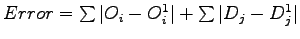
Here the error is calculated as:
 where corresponds to
the actual productions from zone and
where corresponds to
the actual productions from zone and  is the calculated productions
from that zone. Similarly are the actual attractions from the zone
and
is the calculated productions
from that zone. Similarly are the actual attractions from the zone
and  are the calculated attractions from that zone.
The advantages of this method are:
are the calculated attractions from that zone.
The advantages of this method are:
- Simple to understand.
- Preserve observed trip pattern.
- Useful in short term-planning.
The limitations are:
- Depends heavily on the observed trip pattern.
- It cannot explain unobserved trips.
- Do not consider changes in travel cost.
- Not suitable for policy studies like introduction of a mode.
The base year trip matrix for a study area consisting of three zones is given
below.
| |
1 |
2 |
3 |
|
| 1 |
20 |
30 |
28 |
78 |
| 2 |
36 |
32 |
24 |
92 |
| 3 |
22 |
34 |
26 |
82 |
|
88 |
96 |
78 |
252 |
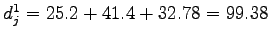
The productions from the zone 1,2 and 3 for the horizon year is expected to
grow to 98, 106, and 122 respectively.
The attractions from these zones are expected to increase to 102, 118, 106
respectively.
Compute the trip matrix for the horizon year using doubly constrained growth
factor model using Furness method.
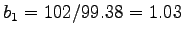
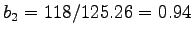
The sum of the attractions in the horizon year, i.e.  = 98+106+122
= 326.
The sum of the productions in the horizon year, i.e.
= 98+106+122
= 326.
The sum of the productions in the horizon year, i.e.  =
102+118+106 = 326.
They both are found to be equal. Therefore we can proceed.
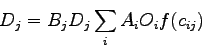
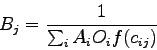
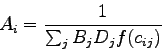
The first step is to fix
=
102+118+106 = 326.
They both are found to be equal. Therefore we can proceed.
The first step is to fix  , and find balancing factor .
 , then find
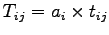
So
 Further
 .
Similarly
.
Similarly
 . etc.
Multiplying with the first row of the matrix, with the second row
and so on, matrix obtained is as shown below.
. etc.
Multiplying with the first row of the matrix, with the second row
and so on, matrix obtained is as shown below.
| |
1 |
2 |
3 |
|
| 1 |
25.2 |
37.8 |
35.28 |
98 |
| 2 |
41.4 |
36.8 |
27.6 |
106 |
| 3 |
32.78 |
50.66 |
38.74 |
122 |
 |
99.38 |
125.26 |
101.62 |
|
|
102 |
118 |
106 |
|
Also
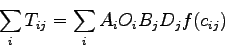
In the second step, find = / and
 .
For example
.
For example
 ,
,
 etc.,
etc.,
 etc.
Also
etc.
Also
 .
The matrix is as shown below:
.
The matrix is as shown below:
| |
1 |
2 |
3 |
|
|
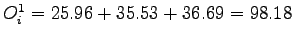
| 1 |
25.96 |
35.53 |
36.69 |
98.18 |
98 |
| 2 |
42.64 |
34.59 |
28.70 |
105.93 |
106 |
| 3 |
33.76 |
47.62 |
40.29 |
121.67 |
122 |
|
1.03 |
0.94 |
1.04 |
|
|
|
102 |
118 |
106 |
|
|
| |
1 |
2 |
3 |
|
|
| 1 |
25.96 |
35.53 |
36.69 |
98.18 |
98 |
| 2 |
42.64 |
34.59 |
28.70 |
105.93 |
106 |
| 3 |
33.76 |
47.62 |
40.29 |
121.67 |
122 |
|
102.36 |
117.74 |
105.68 |
325.78 |
|
|
102 |
118 |
106 |
326 |
|
Therefore error can be computed as ;
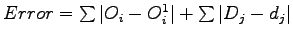
Error =

This model originally generated from an analogy with Newton's gravitational
law.
Newton's gravitational law says,
 Analogous to this,
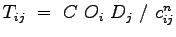 Introducing some balancing factors,
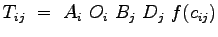 where
where  and
and  are the balancing factors,
  is the generalized
function of the travel cost.
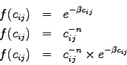
This function is called deterrence function because it represents the
disincentive to travel as distance (time) or cost increases.
Some of the versions of this function are:
is the generalized
function of the travel cost.
This function is called deterrence function because it represents the
disincentive to travel as distance (time) or cost increases.
Some of the versions of this function are:
The first equation is called the exponential function, second one is called
power function where as the third one is a combination of exponential and power
function.
The general form of these functions for different values of their parameters is
as shown in figure.
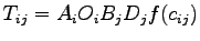
As in the growth factor model, here also we have singly and doubly constrained
models.
The expression
is the classical version of
the doubly constrained model.
Singly constrained versions can be produced by making one set of balancing
factors or equal to one.
Therefore we can treat singly constrained model as a special case which can be
derived from doubly constrained models.
Hence we will limit our discussion to doubly constrained models.
As seen earlier, the model has the functional form,
 |
(4) |
But
 |
(5) |
Therefore,
 |
(6) |
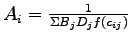
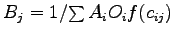
From this we can find the balancing factor as
 |
(7) |
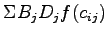
depends on which can be found out by the following equation:
 |
(8) |
We can see that both and are interdependent.
Therefore, through some iteration procedure similar to that of Furness method,
the problem can be solved.
The procedure is discussed below:
- Set = 1, find using equation 8
- Find using equation 7
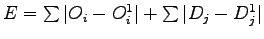
- Compute the error as
where corresponds to the actual productions from zone and is
the calculated productions from that zone. Similarly are the actual
attractions from the zone and are the calculated attractions from
that zone.
- Again set = 1 and find , also find . Repeat these steps
until the convergence is achieved.
The productions from zone 1, 2 and 3 are 98, 106, 122 and attractions to zone
1,2 and 3 are 102, 118, 106.
The function is defined as
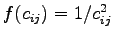 The cost matrix is as shown below
![\begin{displaymath}
\left[ \begin{array}{ccc}
1.0&1.2&1.8 \\
1.2&1.0&1.5 \\
1.8&1.5&1.0 \\
\end{array} \right]
\end{displaymath}](img62.png) |
(9) |
The first step is given in Table 1
Table 1:
Step1: Computation of parameter
|
|
|
 |
|
 |
 |
 |
| |
1 |
1.0 |
102 |
1.0 |
102.00 |
|
|
| 1 |
2 |
1.0 |
118 |
0.69 |
81.42 |
216.28 |
0.00462 |
| |
3 |
1.0 |
106 |
0.31 |
32.86 |
|
|
| |
1 |
1.0 |
102 |
0.69 |
70.38 |
|
|
| 2 |
2 |
1.0 |
118 |
1.0 |
118 |
235.02 |
0.00425 |
| |
3 |
1.0 |
106 |
0.44 |
46.64 |
|
|
| |
1 |
1.0 |
102 |
0.31 |
31.62 |
|
|
| 3 |
2 |
1.0 |
118 |
0.44 |
51.92 |
189.54 |
0.00527 |
| |
3 |
1.0 |
106 |
1.00 |
106 |
|
|
The second step is to find .
This can be found out as
 , where is
obtained from the previous step.
The detailed computation is given in Table 2.
, where is
obtained from the previous step.
The detailed computation is given in Table 2.
Table 2:
Step2: Computation of parameter
|
|
|
|
|
 |
 |
|
| |
1 |
0.00462 |
98 |
1.0 |
0.4523 |
|
|
| 1 |
2 |
0.00425 |
106 |
0.694 |
0.3117 |
0.9618 |
1.0397 |
| |
3 |
0.00527 |
122 |
0.308 |
0.1978 |
|
|
| |
1 |
0.00462 |
98 |
0.69 |
0.3124 |
|
|
| 2 |
2 |
0.00425 |
106 |
1.0 |
0.4505 |
1.0458 |
0.9562 |
| |
3 |
0.00527 |
122 |
0.44 |
0.2829 |
|
|
| |
1 |
0.00462 |
98 |
0.31 |
0.1404 |
|
|
| 3 |
2 |
0.00425 |
106 |
0.44 |
0.1982 |
0.9815 |
1.0188 |
| |
3 |
0.00527 |
122 |
1.00 |
0.6429 |
|
|
The function can be written in the matrix form as:
![\begin{displaymath}
\left[ \begin{array}{ccc} 1.0&0.69&0.31 \\
0.69&1.0&0.44 \\
0.31&0.44&1.0 \\
\end{array} \right]
\end{displaymath}](img70.png) |
(10) |
Then can be computed using the formula
 |
(11) |
For eg,
 .
is the actual productions from the zone and is the computed ones.
Similar is the case with attractions also. The results are shown in table 3.
.
is the actual productions from the zone and is the computed ones.
Similar is the case with attractions also. The results are shown in table 3.
Table 3:
Step3: Final Table
| |
1 |
2 |
3 |
|
|
|
| 1 |
48.01 |
35.24 |
15.157 |
0.00462 |
98 |
98.407 |
| 2 |
32.96 |
50.83 |
21.40 |
0.00425 |
106 |
105.19 |
| 3 |
21.14 |
31.919 |
69.43 |
0.00527 |
122 |
122.489 |
|
1.0397 |
0.9562 |
1.0188 |
|
|
|
|
102 |
118 |
106 |
|
|
|
|
102.11 |
117.989 |
105.987 |
|
|
|
is the actual productions from the zone and is the computed ones.
Similar is the case with attractions also.
Therefore error can be computed as ;

The second stage of travel demand modeling is the trip distribution.
Trip matrix can be used to represent the trip pattern of a study area.
Growth factor methods and gravity model are used for computing the trip matrix.
Singly constrained models and doubly constrained growth factor models are discussed.
In gravity model, considering singly constrained model as a special case of
doubly constrained model, doubly constrained model is explained in detail.
The trip productions from zones 1, 2 and 3 are 110, 122 and 114
respectively and the trip attractions to these zones are 120,108, and 118
respectively.
The cost matrix is given below.
The function

Compute the trip matrix using doubly constrained gravity model.
Provide one complete iteration.
The first step is given in Table 4
Table 4:
Step1: Computation of parameter
|
|
|
|
|
|
|
|
| |
1 |
1.0 |
120 |
1.0 |
120.00 |
|
|
| 1 |
2 |
1.0 |
108 |
0.833 |
89.964 |
275.454 |
0.00363 |
| |
3 |
1.0 |
118 |
0.555 |
65.49 |
|
|
| |
1 |
1.0 |
120 |
0.833 |
99.96 |
|
|
| 2 |
2 |
1.0 |
108 |
1.0 |
108 |
286.66 |
0.00348 |
| |
3 |
1.0 |
118 |
0.667 |
78.706 |
|
|
| |
1 |
1.0 |
120 |
0.555 |
66.60 |
|
|
| 3 |
2 |
1.0 |
108 |
0.667 |
72.036 |
256.636 |
0.00389 |
| |
3 |
1.0 |
118 |
1.00 |
118 |
|
|
The second step is to find .
This can be found out as
, where is
obtained from the previous step.
Table 5:
Step2: Computation of parameter
|
|
|
|
|
|
|
|
| |
1 |
0.00363 |
110 |
1.0 |
0.3993 |
|
|
| 1 |
2 |
0.00348 |
122 |
0.833 |
0.3536 |
0.9994 |
1.048 |
| |
3 |
0.00389 |
114 |
0.555 |
0.2465 |
|
|
| |
1 |
0.00363 |
110 |
0.833 |
0.3326 |
|
|
| 2 |
2 |
0.00348 |
122 |
1.0 |
0.4245 |
1.05 |
0.9494 |
| |
3 |
0.00389 |
114 |
0.667 |
0.2962 |
|
|
| |
1 |
0.00363 |
110 |
0555 |
0.2216 |
|
|
| 3 |
2 |
0.00348 |
122 |
0.667 |
0.2832 |
0.9483 |
1.054 |
| |
3 |
0.00389 |
114 |
1.00 |
0.44346 |
|
|
The function can be written in the matrix form as:
![\begin{displaymath}
\left[ \begin{array}{ccc} 1.0 & 0.833 &0.555 \\
0.833 &1.0 & 0.667 \\
0.555 & 0.667 & 1.0 \\
\end{array} \right]
\end{displaymath}](img77.png) |
(12) |
Then can be computed using the formula
|
(13) |
For eg,
.
is the actual productions from the zone and is the computed ones.
Similar is the case with attractions also.
This step is given in Table 6
Table 6:
Step 3: Final Table
| |
1 |
2 |
3 |
|
|
|
| 1 |
48.01 |
34.10 |
27.56 |
0.00363 |
110 |
109.57 |
| 2 |
42.43 |
43.53 |
35.21 |
0.00348 |
122 |
121.17 |
| 3 |
29.53 |
30.32 |
55.15 |
0.00389 |
114 |
115 |
|
1.048 |
0.9494 |
1.054 |
|
|
|
|
120 |
108 |
118 |
|
|
|
|
119.876 |
107.95 |
117.92 |
|
|
|
is the actual productions from the zone and is the computed ones.
Similar is the case with attractions also.
Therefore error can be computed as ;

Prof. Tom V. Mathew
2011-08-10
![\begin{eqnarray*}
\left[ \begin{array}{ccc} 1.0&1.2&1.8 \\
1.2&1.0&1.5 \\
1.8&1.5&1.0 \\
\end{array} \right]
\end{eqnarray*}](img76.png)