Modal Split
Lecture notes in Transportation Systems Engineering
August 8, 2011
The third stage in travel demand modeling is modal split.
The trip matrix or O-D matrix obtained from the trip distribution is sliced
into number of matrices representing each mode.
First the significance and factors affecting mode choice problem will be
discussed.
Then a brief discussion on the classification of mode choice will be made.
Two types of mode choice models will be discussed in detail. ie binary mode
choice and multinomial mode choice.
The chapter ends with some discussion on future topics in mode choice problem.
The choice of transport mode is probably one of the most important classic
models in transport planning.
This is because of the key role played by public transport in policy making.
Public transport modes make use of road space more efficiently than private
transport.
Also they have more social benefits like if more people begin to use public
transport , there will be less congestion on the roads and the accidents will be
less.
Again in public transport, we can travel with low cost.
In addition, the fuel is used more efficiently.
Main characteristics of public transport is that they will have some
particular schedule, frequency etc.
On the other hand, private transport is highly flexible.
It provides more comfortable and convenient travel.
It has better accessibility also.
The issue of mode choice, therefore, is probably the single most important
element in transport planning and policy making.
It affects the general efficiency with which we can travel in urban areas.
It is important then to develop and use models which are sensitive to those
travel attributes that influence individual choices of mode.
The factors may be listed under three groups:
- Characteristics of the trip maker : The following features are
found to be important:
- car availability and/or ownership;
- possession of a driving license;
- household structure (young couple, couple with children, retired people
etc.);
- income;
- decisions made elsewhere, for example the need to use a car at work, take
children to school, etc;
- residential density.
- Characteristics of the journey: Mode choice is strongly influenced
by:
- The trip purpose; for example, the journey to work is normally easier to
undertake by public transport than other journeys because of its regularity and
the adjustment possible in the long run;
- Time of the day when the journey is undertaken.
- Late trips are more difficult to accommodate by public transport.
- Characteristics of the transport facility: There are two types of
factors.One is quantitative and the other is qualitative.
Quantitative factors are:
- relative travel time: in-vehicle, waiting and walking times by each mode;
- relative monetary costs (fares, fuel and direct costs);
- availability and cost of parking
Qualitative factors which are less easy to measure are:
- comfort and convenience
- reliability and regularity
- protection, security
A good mode choice should include the most important of these factors.
Traditionally, the objective of transportation planning was to forecast the
growth in demand for car trips so that investment could be planned to meet the
demand.
When personal characteristics were thought to be the most important
determinants of mode choice, attempts were made to apply modal-split models
immediately after trip generation.
Such a model is called trip-end modal split model.
In this way different characteristics of the person could be preserved and used
to estimate modal split.
The modal split models of this time related the choice of mode only to features
like income, residential density and car ownership.
The advantage is that these models could be very accurate in the short run, if
public transport is available and there is little congestion.
Limitation is that they are insensitive to policy decisions example: Improving
public transport, restricting parking etc. would have no effect on modal split
according to these trip-end models.
This is the post-distribution model; that is modal split is applied after the
distribution stage.
This has the advantage that it is possible to include the characteristics of
the journey and that of the alternative modes available to undertake them.
It is also possible to include policy decisions.
This is beneficial for long term modeling.
Mode choice could be aggregate if they are based on zonal and
inter-zonal information.
They can be called disaggregate if they are based on household or
individual data.
Binary logit model is the simplest form of mode choice, where the travel choice
between two modes is made.
The traveler will associate some value for the utility of each mode.
if the utility of one mode is higher than the other, then that mode is chosen.
But in transportation, we have disutility also.
The disutility here is the travel cost.
This can be represented as
 |
(1) |
where  is the in-vehicle travel time between
  and
and  ,
,  is the walking time to and from stops,
  is the waiting time at stops,
 is the fare charged to travel between and ,
  is the
parking cost, and
is the
parking cost, and  is a parameter representing comfort and convenience.
If the travel cost is low, then that mode has more probability of being chosen.
Let there be two modes (m=1,2) then the proportion of trips by mode 1 from zone
to zone is(
is a parameter representing comfort and convenience.
If the travel cost is low, then that mode has more probability of being chosen.
Let there be two modes (m=1,2) then the proportion of trips by mode 1 from zone
to zone is( )
Let
)
Let  be the cost of traveling from zone to zone using the
mode 1, and
be the cost of traveling from zone to zone using the
mode 1, and  be the cost of traveling from zone to zone by
mode 2,there are three cases:
be the cost of traveling from zone to zone by
mode 2,there are three cases:
- if - is positive, then mode 1 is chosen.
- if - is negative, then mode 2 is chosen.
- if - = 0 , then both modes have equal probability.
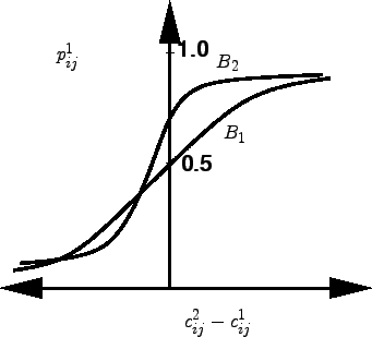
This relationship is normally expressed by a logit curve as shown in figure
1
Therefore the proportion of trips by mode 1 is given by
 |
(2) |
This functional form is called logit, where  is called
the generalized cost and
is called
the generalized cost and  is the parameter for calibration.
The graph in figure 1 shows the proportion of trips by mode 1
(
is the parameter for calibration.
The graph in figure 1 shows the proportion of trips by mode 1
(
 ) against cost difference.
Figure 1:
logit function
 |
Let the number of trips from zone to zone is 5000, and two modes are
available which has the characteristics given in Table 1.
Compute the trips made by mode bus, and the fare that is collected from the
mode bus.
If the fare of the bus is reduced to 6, then find the fare collected.
Table 1:
Trip characterisitcs
| |
 |
 |
 |
 |
|
| car |
20 |
- |
18 |
4 |
|
| bus |
30 |
5 |
3 |
9 |
|
 |
0.03 |
0.04 |
0.06 |
0.1 |
0.1 |
Table 2:
Binary logit model example: solution
| |
|
|
|
|
|
|
 |
 |
| ar |
20 |
- |
18 |
4 |
|
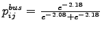
2.08 |
.52 |
2600 |
| bus |
30 |
5 |
3 |
9 |
|
2.18 |
.475 |
2400 |
|
.03 |
.04 |
.06 |
.1 |
.1 |
|
|
|
The base case is given below.
Cost of travel by car (Equation)=
 = 2.08
Cost of travel by bus (Equation)=
= 2.08
Cost of travel by bus (Equation)=
 = 2.18
Probability of choosing mode car (Equation)=
= 2.18
Probability of choosing mode car (Equation)=
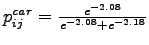 = 0.52
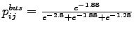
Probability of choosing mode bus (Equation)=
= 0.52
Probability of choosing mode bus (Equation)=
 = 0.475
Proportion of trips by car =
= 0.475
Proportion of trips by car =  = 5000
 0.52 = 2600
Proportion of trips by bus =
0.52 = 2600
Proportion of trips by bus =  = 50000.475 = 2400
Fare collected from bus =
= 50000.475 = 2400
Fare collected from bus =
 = 24009 =
21600
= 24009 =
21600
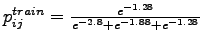
When the fare of bus gets reduced to 6,
Cost function for bus=
 = 1.88
Probability of choosing mode bus (Equation)=
= 1.88
Probability of choosing mode bus (Equation)=
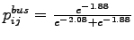 = 0.55
Proportion of trips by bus = = 50000.55 = 2750
Fare collected from the bus
= 27506 =
16500
= 0.55
Proportion of trips by bus = = 50000.55 = 2750
Fare collected from the bus
= 27506 =
16500
The results are tabulated in table
The binary model can easily be extended to multiple modes.
The equation for such a model can be written as:
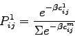 |
(3) |
Let the number of trips from to is 5000, and three modes are available
which has the characteristics given in Table 3:
Compute the trips made by the three modes and the fare required to travel by
each mode.
Table 3:
Trip characteristics
| |
 |
 |
|
|
 |
| coefficient |
0.03 |
0.04 |
0.06 |
0.1 |
0.1 |
| car |
20 |
- |
- |
18 |
4 |
| bus |
30 |
5 |
3 |
6 |
- |
| train |
12 |
10 |
2 |
4 |
- |
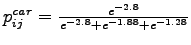
Cost of travel by car (Equation)=
 = 2.8
Cost of travel by bus (Equation)=
= 1.88
Cost of travel by train (Equation)=
= 2.8
Cost of travel by bus (Equation)=
= 1.88
Cost of travel by train (Equation)=
 = 1.28
Probability of choosing mode car (Equation)
= 1.28
Probability of choosing mode car (Equation)
 = 0.1237
Probability of choosing mode bus (Equation
= 0.1237
Probability of choosing mode bus (Equation
 = 0.3105
Probability of choosing mode train (Equation)=
= 0.3105
Probability of choosing mode train (Equation)=
 = 0.5657
Proportion of trips by car, = 50000.1237 = 618.5
Proportion of trips by bus, = 50000.3105 = 1552.5
Similarly, proportion of trips by train,
= 0.5657
Proportion of trips by car, = 50000.1237 = 618.5
Proportion of trips by bus, = 50000.3105 = 1552.5
Similarly, proportion of trips by train,
 =
50000.5657 = 2828.5
We can put all this in the form of a table as shown below 4:
=
50000.5657 = 2828.5
We can put all this in the form of a table as shown below 4:
Table 4:
Multinomial logit model problem: solution
| |
|
|
|
|
|
 |
 |
|
|
| coeff |
0.03 |
0.04 |
0.06 |
0.1 |
0.1 |
- |
- |
- |
- |
| car |
20 |
- |
- |
18 |
4 |
2.8 |
0.06 |
0.1237 |
618.5 |
| bus |
30 |
5 |
3 |
6 |
- |
1.88 |
0.15 |
0.3105 |
1552.5 |
| train |
12 |
10 |
2 |
4 |
- |
1.28 |
0.28 |
0.5657 |
2828.5 |
- $$
Fare collected from the mode bus =
=
1552.56 = 9315
- $$
Fare collected from mode train =
 =
2828.54 = 11314
=
2828.54 = 11314
Modal split is the third stage of travel demand modeling.
The choice of mode is influenced by various factors.
Different types of modal split models are there.
Binary logit model and multinomial logit model are dealt in detail
in this chapter.
- The total number of trips from zone to zone is 4200.
Currently all trips are made by car. Government has two alternatives- to
introduce a train or a bus.
The travel characteristics and respective coefficients are given in table 5.
Decide the best alternative in terms of trips carried.
Table 5:
Trip characteristics
| |
|
|
|
|
|
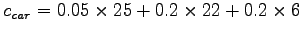
| coefficient |
0.05 |
0.04 |
0.07 |
0.2 |
0.2 |
| car |
25 |
- |
- |
22 |
6 |
| bus |
35 |
8 |
6 |
8 |
- |
| train |
17 |
14 |
5 |
6 |
- |
First, use binary logit model to find the trips when there is only car and
bus.
Then, again use binary logit model to find the trips when there is only car and
train.
Finally compare both and see which alternative carry maximum trips.
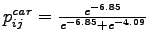
Cost of travel by car=
 = 6.85
Cost of travel by bus=
= 6.85
Cost of travel by bus=
 = 4.09
Cost of travel by trai=
= 4.09
Cost of travel by trai=
 = 2.96
Case 1: Considering introduction of bus,
Probability of choosing car,
= 2.96
Case 1: Considering introduction of bus,
Probability of choosing car,
 = 0.059
Probability of choosing bus,
= 0.059
Probability of choosing bus,
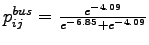 = 0.9403
Case 2: Considering introduction of train,
Probability of choosing car
= 0.9403
Case 2: Considering introduction of train,
Probability of choosing car
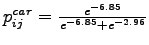 = 0.02003
Probability of choosing train
= 0.02003
Probability of choosing train
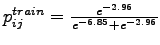 = 0.979
Trips carried by each mode
= 0.979
Trips carried by each mode
Case 1:
= 42000.0596 = 250.32
= 42000.9403 = 3949.546
Case 2:
= 42000.02 = 84.00
= 42000.979 = 4115.8
Hence train will attract more trips, if it is introduced.
Prof. Tom V. Mathew
2011-08-08