Trip Assignment
Lecture notes in Transportation Systems Engineering
August 23, 2011
The process of allocating given set of trip interchanges to the specified
transportation system is usually referred to as trip assignment or traffic assignment.
The fundamental aim of the traffic assignment process is to reproduce on the
transportation system, the pattern of vehicular movements which would be
observed when the travel demand represented by the trip matrix, or matrices, to
be assigned is satisfied.
The major aims of traffic assignment procedures are:
- To estimate the volume of traffic on the links of the network and obtain
aggregate network measures.
- To estimate inter zonal travel cost.
- To analyze the travel pattern of each origin to destination(O-D) pair.
- To identify congested links and to collect traffic data useful for the
design of future junctions.
As the flow increases towards the capacity of the stream, the average stream
speed reduces from the free flow speed to the speed corresponding to the
maximum flow.
This can be seen in the graph shown below.
Figure 1:
Two Link Problem with constant travel time function
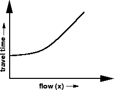 |
That means traffic conditions worsen and congestion starts developing.
The inter zonal flows are assigned to the minimum paths computed on the basis of
free-flow link impedances (usually travel time).
But if the link flows were at the levels dictated by the assignment, the link
speeds would be lower and the link travel time would be higher than those
corresponding to the free flow conditions.
So the minimum path computed prior to the trip assignment will not be the
minimum after the trips ae assigned.
A number of iterative procedures are done to converge this difference.
The relation between the link flow and link impedance is called the link cost
function and is given by the equation as shown below:
![\begin{displaymath}
t = t_0 {[1+{\alpha} {{(\frac{x}{k})}^{\beta}}]}
% Link Travel Time Functin
\end{displaymath}](img2.png) |
(1) |
where  and
and  is the travel time and flow, respectively on the link,
  is the free flow travel time, and k is the practical capacity.
The parameters
is the free flow travel time, and k is the practical capacity.
The parameters  and
and  are specific the type of link and is to be
calibrated from the field data.
In the absense of any field data, following values could the assumed: = 0.15, and = 4.0.
are specific the type of link and is to be
calibrated from the field data.
In the absense of any field data, following values could the assumed: = 0.15, and = 4.0.
The types of traffic assignment models are all-or-nothing assignment
(AON), incremental assignment, capacity restraint assignment, user equilibrium
assignment (UE), stochastic user equilibrium assignment (SUE), system optimum
assignment (SO), etc.
The frequently used models all-or-nothing, user equilibrium, and system optimum
will be discussed in detail here.
In this method the trips from any origin zone to any destination zone are
loaded onto a single, minimum cost, path between them.
This model is unrealistic as only one path between every O-D pair is utilized
even if there is another path with the same or nearly same travel cost.
Also, traffic on links is assigned without consideration of whether or not
there is adequate capacity or heavy congestion; travel time is a fixed input
and does not vary depending on the congestion on a link.
However, this model may be reasonable in sparse and uncongested networks where
there are few alternative routes and they have a large difference in travel
cost.
This model may also be used to identify the desired path : the path
which the drivers would like to travel in the absence of congestion.
In fact, this model's most important practical application is that it acts as a
building block for other types of assignment techniques.It has a limitation
that it ignores the fact that link travel time is a function of link volume and
when there is congestion or that multiple paths are used to carry traffic.
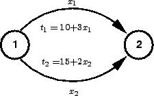
To demonstrate how this assignment works, an example network is considered.
This network has two nodes having two paths as links.
Let us suppose a case where travel time is not a function of flow as shown in
other words it is constant as shown in the figure below.
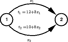
Figure 2:
Two Link Problem with constant travel time function
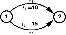 |
The travel time functions for both the links is given by:


and total flows from 1 to 2 is given by.

Since the shortest path is Link 1 all flows are assigned to it making  =12
and
=12
and  = 0.
= 0.
The user equilibrium assignment is based on Wardrop's first principle, which
states that no driver can unilaterally reduce his/her travel costs by
shifting to another route.
User Equilibrium (UE) conditions can be written for a given O-D pair as:
 |
(2) |
 |
(3) |
where  is the flow on path
  ,
,  is the travel cost on
path , and
is the travel cost on
path , and  is the minimum cost.
Equation 3 can have two states.
is the minimum cost.
Equation 3 can have two states.
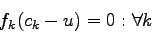
- If
 = 0, from equation 2
  0.
This means that all used paths will have same travel time.
0.
This means that all used paths will have same travel time.
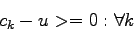
- If
 0, then from equation 2 = 0.
This means that all unused paths will have travel time greater than the minimum
cost path. where is the flow on path , is the travel cost on
path , and is the minimum cost.
- The user has perfect knowledge of the path cost.
- Travel time on a given link is a function of the flow on that link only.
- Travel time functions are positive and increasing.
The solution to the above equilibrium conditions given by the solution of an
equivalent nonlinear mathematical optimization program,
where is the path,  equilibrium flows in link a,
  travel
time on link a,
travel
time on link a,  flow on path k connecting O-D pair
r-s,
flow on path k connecting O-D pair
r-s,  trip rate between r and sand
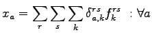
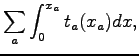
 is a
definitional constraint and is given by
is a
definitional constraint and is given by
 |
(5) |
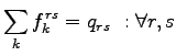
The equations above are simply flow conservation equations and non negativity
constraints, respectively.
These constraints naturally hold the point that minimizes the objective
function.
These equations state user equilibrium principle.The path connecting O-D pair
can be divided into two categories : those carrying the flow and those not
carrying the flow on which the travel time is greater than (or equal to)the
minimum O-D travel time.
If the flow pattern satisfies these equations no motorist can better off by
unilaterally changing routes.
All other routes have either equal or heavy travel times.
The user equilibrium criteria is thus met for every O-D pair.
The UE problem is convex because the link travel time functions are
monotonically
increasing function, and the link travel time a particular link is independent
of the flow and other links of the networks. To solve such convex problem
Frank Wolfe algorithm is useful.
Let us suppose a case where travel time is not a function of flow as shown in
other words it is constant as shown in the figure below.
Figure 3:
Two Link Problem with constant travel time function
 |
Substituting the travel time in equation yield to
subject to
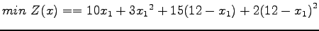
Substituting 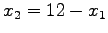 , in the above formulation will yield the
unconstrained formulation as below :
, in the above formulation will yield the
unconstrained formulation as below :
Differentiate the above equation and equate to zero, and solving for
and then leads to the solution = 5.8, = 6.2.
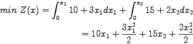
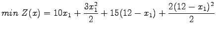
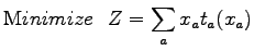
The system optimum assignment is based on Wardrop's second principle, which
states that drivers cooperate with one another in order to minimize total
system travel time.
This assignment can be thought of as a model in which congestion is minimized
when drivers are told which routes to use.
Obviously, this is not a behaviorally realistic model, but it can be useful to
transport planners and engineers, trying to manage the traffic to minimize
travel costs and therefore achieve an optimum social equilibrium.
 |
|
|
(6) |
subject to
equilibrium flows in link a, travel time on link
a, flow on path k connecting O-D pair r-s, trip
rate between r and s.
To demonstrate how the assignment works, an example network is considered.
This network has two nodes having two paths as links. Let us suppose a case
where travel time is not a function of flow or in other words it is constant as
shown in the figure below.
Figure 4:
Two Link Problem with constant travel time function
|
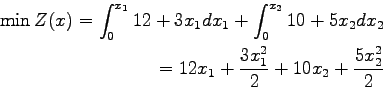
Substituting the travel time in equation , we get the following:
 |
|
|
(11) |
 |
|
|
(12) |
Substituting 
 |
|
|
(13) |
Differentiate the above equation to zero, and solving for and then
leads to the solution
= 5.3,= 6.7
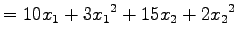
which gives Z(x) = 327.55
Let us discuss briefly some other assignments like incremental assignment, capacity restraint assignment, stochastic user equilibrium assignment and dynamic assignment.
Incremental assignment is a process in which fractions of traffic volumes are
assigned in steps.In each step, a fixed proportion of total demand is assigned,
based on all-or-nothing assignment.
After each step, link travel times are recalculated based on link volumes.
When there are many increments used, the flows may resemble an equilibrium
assignment ; however, this method does not yield an equilibrium solution.
Consequently, there will be inconsistencies between link volumes and travel
times that can lead to errors in evaluation measures.
Also, incremental assignment is influenced by the order in which volumes for
O-D pairs are assigned, raising the possibility of additional bias in results.
Capacity restraint assignment attempts to approximate an equilibrium solution
by iterating between all-or-nothing traffic loadings and recalculating link
travel times based on a congestion function that reflects link capacity.
Unfortunately, this method does not converge and can flip-flop back and forth
in loadings on some links.
User equilibrium assignment procedures based on Wardrop's principle assume that
all drivers perceive costs in an identical manner.
A solution to assignment problem on this basis is an assignment such that no
driver can reduce his journey cost by unilaterally changing route.
Van Vilet considered as stochastic assignment models, all those models which
explicitly allows non minimum cost routes to be selected.
Virtually all such models assume that drivers perception of costs on any given
route are not identical and that the trips between each O-D pair are divided
among the routes with the most cheapest route attracting most trips.
They have important advantage over other models because they load many routes
between individual pairs of network nodes in a single pass through the tree
building process,the assignments are more stable and less sensitive to slight
variations in network definitions or link costs to be independent of flows and
are thus most appropriate for use in uncongested traffic conditions such as in
off peak periods or lightly trafficked rural areas.
Dynamic user equilibrium,expressed as an extension of Wardrop's user
equilibrium principle, may be defined as the state of equilibrium which arises
when no driver can reduce his disutility of travel by choosing a new route or
departure time,where disutility includes, schedule delay in addition in to costs
generally considered. Dynamic stochastic equilibrium may be similarly defined
in terms of perceived utility of travel.
The existence of such equilibrium in complex networks has not been proven
theoretical and even if they exist the question of uniqueness remains open.
Traffic assignment is the last stage of traffic demand modeling.
There are different types of traffic assignment models.
All-or-nothing, User-equilibrium, and System-optimum assignment models are
the commonly used models.
All-or-nothing model is an unrealistic model since only one path between every
O-D pair is utilised and they can give satisfactory results only when the network
is least congested.
User-equilibrium assignment is based on Wardrop's first principle and it's conditions
are based on certain assumptions.
Wardrop's second principle is utilized by System-optimum method and it tries to
minimise the congestion by giving prior information to drivers regarding the respective
routes to be chosen.
Other assignment models are also briefly explained.
Calculate the system travel time and link flows by doing user equilibrium
assignment for the network in the given figure 5.
Verify that the flows are at user equilibrium.
Figure 5:
Two link problem with constant travel time
 |
Substituting the travel time in the respective equation yield to
subject
to
Substituting , in the above formulation will yield the
unconstrained formulation as below :
Differentiate the above equation and equating to zero,
Travel times are
It follows that the travel times are at user equilibrium.
Prof. Tom V. Mathew
2011-08-23