Microscopic traffic flow modeling
Lecture notes in Transportation Systems Engineering
September 8, 2011
Macroscopic modeling looks at traffic flow from a global perspective, whereas
microscopic modeling, as the term suggests, gives attention to the details of
traffic flow and the interactions taking place within it.
This chapter gives an overview of microscopic approach to modeling traffic and
then elaborates on the various concepts associated with it.
A microscopic model of traffic flow attempts to analyze the flow of
traffic by modeling driver-driver and driver-road interactions within a
traffic stream which respectively analyzes the interaction between a driver and
another driver on road and of a single driver on the different features of a
road.
Many studies and researches were carried out on driver's behavior in different
situations like a case when he meets a static obstacle or when he meets a
dynamic obstacle.
Several studies are made on modeling driver behavior in another following car
and such studies are often referred to as car following theories of vehicular
traffic.
Longitudinal spacing of vehicles are of particular importance from the points
of view of safety, capacity and level of service.
The longitudinal space occupied by a vehicle depend on the physical dimensions
of the vehicles as well as the gaps between vehicles.
For measuring this longitudinal space, two microscopic measures are used-
distance headway and distance gap.
Distance headway is defined as the distance from a selected point (usually
front bumper) on the lead vehicle to the corresponding point on the following
vehicles.
Hence, it includes the length of the lead vehicle and the gap length between
the lead and the following vehicles.
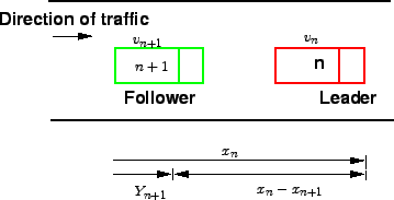
Before going in to the details, various notations used in car-following models
are discussed here with the help of figure 1.
The leader vehicle is denoted as  and the following vehicle as
  . Two
characteristics at an instant
. Two
characteristics at an instant  are of importance; location and speed.
Location and speed of the lead vehicle at time instant are represented by
are of importance; location and speed.
Location and speed of the lead vehicle at time instant are represented by
 and
and  respectively. Similarly, the location and speed of the
follower are denoted by
respectively. Similarly, the location and speed of the
follower are denoted by  and
and  respectively.
The following vehicle is assumed to accelerate at time
respectively.
The following vehicle is assumed to accelerate at time  and not at
, where
and not at
, where  is the interval of time required for a driver to react to
a changing situation.
The gap between the leader and the follower vehicle is therefore
is the interval of time required for a driver to react to
a changing situation.
The gap between the leader and the follower vehicle is therefore
 .
.
Figure 1:
Notation for car following model
 |
Car following theories describe how one vehicle follows another vehicle in an
uninterrupted flow. Various models were formulated to represent how a driver
reacts to the changes in the relative positions of the vehicle ahead.
Models like Pipes, Forbes, General Motors and Optimal velocity model are worth
discussing.
The basic assumption of this model is ``A good rule for following another
vehicle at a safe distance is to allow yourself at least the length of a car
between your vehicle and the vehicle ahead for every ten miles per hour of
speed at which you are traveling"
According to Pipe's car-following model, the minimum safe distance headway
increases linearly with speed.
A disadvantage of this model is that at low speeds, the minimum headways
proposed by the theory are considerably less than the corresponding field
measurements.
In this model, the reaction time needed for the following vehicle to perceive
the need to decelerate and apply the brakes is considered.
That is, the time gap between the rear of the leader and the front of the
follower should always be equal to or greater than the reaction time.
Therefore, the minimum time headway is equal to the reaction time (minimum time
gap) and the time required for the lead vehicle to traverse a distance
equivalent to its length.
A disadvantage of this model is that, similar to Pipe's model, there is a wide
difference in the minimum distance headway at low and high speeds.
The General Motors' model is the most popular of the car-following theories
because of the following reasons:
- Agreement with field data; the simulation models developed based on
General motors' car following models shows good correlation to the field data.
- Mathematical relation to macroscopic model; Greenberg's logarithmic
model for speed-density relationship can be derived from General motors car
following model.
In car following models, the motion of individual vehicle is governed by an
equation, which is analogous to the Newton's Laws of motion.
In Newtonian mechanics, acceleration can be regarded as the response of the
particle to stimulus it receives in the form of force which includes
both the external force as well as those arising from the interaction with all
other particles in the system.
This model is the widely used and will be discussed in detail later.
The concept of this model is that each driver tries to achieve an optimal
velocity based on the distance to the preceding vehicle and the speed
difference between the vehicles.
This was an alternative possibility explored recently in car-following models.
The formulation is based on the assumption that the desired speed
 depends on the distance headway of the th vehicle.
i.e.
depends on the distance headway of the th vehicle.
i.e.
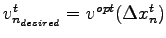 where
where  is the optimal velocity function which is a function of the
instantaneous distance headway
is the optimal velocity function which is a function of the
instantaneous distance headway  .
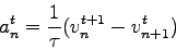
Therefore
.
Therefore  is given by
![\begin{displaymath}
{a_n^t} =[1/\tau][V^{opt}{({\Delta}x_n^t)}-{v_n^t}]
\end{displaymath}](img17.png) |
(1) |
where
 is called as sensitivity coefficient. In short, the
driving strategy of
is called as sensitivity coefficient. In short, the
driving strategy of  vehicle is that, it tries to maintain a safe speed
which inturn depends on the relative position, rather than relative speed.
vehicle is that, it tries to maintain a safe speed
which inturn depends on the relative position, rather than relative speed.
The basic philosophy of car following model is from Newtonian mechanics, where
the acceleration may be regarded as the response of a matter to the stimulus it
receives in the form of the force it receives from the interaction with other
particles in the system.
Hence, the basic philosophy of car-following theories can be summarized by the
following equation
![\begin{displaymath}[{\mathrm{Response}}]_n \alpha [{\mathrm Stimulus}]_n
\end{displaymath}](img20.png) |
(2) |
for the nth vehicle (n=1, 2, ...).
Each driver can respond to the surrounding traffic conditions only by
accelerating or decelerating the vehicle.
As mentioned earlier, different theories on car-following have arisen because
of the difference in views regarding the nature of the stimulus.
The stimulus may be composed of the speed of the vehicle, relative speeds,
distance headway etc, and hence, it is not a single variable, but a function
and can be represented as,
 |
(3) |
where  is the stimulus function that depends on the speed of the
current vehicle, relative position and speed with the front vehicle.
is the stimulus function that depends on the speed of the
current vehicle, relative position and speed with the front vehicle.
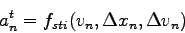
The car following model proposed by General motors is based on follow-the
leader concept.
This is based on two assumptions; (a) higher the speed of the vehicle, higher
will be the spacing between the vehicles and (b) to avoid collision, driver
must maintain a safe distance with the vehicle ahead.
Let
 is the gap available for
  vehicle, and
let
vehicle, and
let
 is the safe distance,
  and
and  are the
velocities, the gap required is given by,
are the
velocities, the gap required is given by,
 |
(4) |
where  is a sensitivity coefficient.
The above equation can be written as
is a sensitivity coefficient.
The above equation can be written as
 |
(5) |
Differentiating the above equation with respect to time, we get
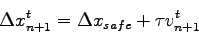
General Motors has proposed various forms of sensitivity coefficient term
resulting in five generations of models.
The most general model has the form,
![\begin{displaymath}
a^t_{n+1} =
\left[\frac{\alpha_{l,m}{(v^t_{n+1}})^m}{{(x^t_n-x^t_{n+1}})^{l}}\right]\left[v_n^{t}-v^t_{n+1}\right]
\end{displaymath}](img32.png) |
(6) |
where  is a distance headway exponent and can take values from +4 to -1,
  is a speed exponent and can take values from -2 to +2, and
  is a
sensitivity coefficient.
These parameters are to be calibrated using field data.
This equation is the core of traffic simulation models.
is a
sensitivity coefficient.
These parameters are to be calibrated using field data.
This equation is the core of traffic simulation models.
In computer, implementation of the simulation models, three things need to be
remembered:
- A driver will react to the change in speed of the front vehicle after a
time gap called the reaction time during which the follower perceives the
change in speed and react to it.
- The vehicle position, speed and acceleration will be updated at certain
time intervals depending on the accuracy required.
Lower the time interval, higher the accuracy.
- Vehicle position and speed is governed by Newton's laws of motion, and
the acceleration is governed by the car following model.
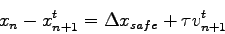
Therefore, the governing equations of a traffic flow can be developed as below.
Let  is the reaction time, and
  is the updation time, the
governing equations can be written as,
is the updation time, the
governing equations can be written as,
The equation 7 is a simulation version of the Newton's simple law of
motion  and equation 8 is the simulation version of the
Newton's another equation
and equation 8 is the simulation version of the
Newton's another equation
 .
The acceleration of the follower vehicle depends upon the relative velocity of
the leader and the follower vehicle, sensitivity coefficient and the gap
between the vehicles.
.
The acceleration of the follower vehicle depends upon the relative velocity of
the leader and the follower vehicle, sensitivity coefficient and the gap
between the vehicles.
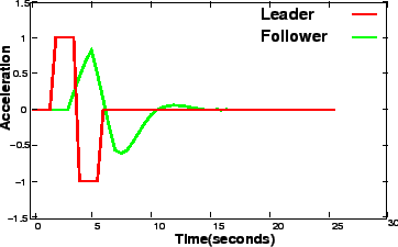
Let a leader vehicle is moving with zero acceleration for two seconds from time
zero.
Then he accelerates by 1  for 2 seconds, then decelerates by 1for
2 seconds.
The initial speed is 16 m/s and initial location is 28 m from datum.
A vehicle is following this vehicle with initial speed 16 m/s, and position
zero.
Simulate the behavior of the following vehicle using General Motors' Car
following model (acceleration, speed and position) for 7.5 seconds.
Assume the parameters l=1, m=0 , sensitivity coefficient (
for 2 seconds, then decelerates by 1for
2 seconds.
The initial speed is 16 m/s and initial location is 28 m from datum.
A vehicle is following this vehicle with initial speed 16 m/s, and position
zero.
Simulate the behavior of the following vehicle using General Motors' Car
following model (acceleration, speed and position) for 7.5 seconds.
Assume the parameters l=1, m=0 , sensitivity coefficient ( ) = 13,
reaction time as 1 second and scan interval as 0.5 seconds.
) = 13,
reaction time as 1 second and scan interval as 0.5 seconds.
The first column shows the time in seconds.
Column 2, 3, and 4 shows the acceleration, velocity and distance of the leader
vehicle.
Column 5,6, and 7 shows the acceleration, velocity and distance of the follower
vehicle.
Column 8 gives the difference in velocities between the leader and follower
vehicle denoted as  .
Column 9 gives the difference in displacement between the leader and follower
vehicle denoted as
.
Column 9 gives the difference in displacement between the leader and follower
vehicle denoted as  .
Note that the values are assumed to be the state at the beginning of that time
interval.
At time t=0, leader vehicle has a velocity of 16 m/s and located at a distance
of 28 m from a datum.
The follower vehicle is also having the same velocity of 16 m/s and located at
the datum.
Since the velocity is same for both, = 0.
At time t = 0, the leader vehicle is having acceleration zero, and hence has
the same speed.
The location of the leader vehicle can be found out from equation as, x = 28+16
.
Note that the values are assumed to be the state at the beginning of that time
interval.
At time t=0, leader vehicle has a velocity of 16 m/s and located at a distance
of 28 m from a datum.
The follower vehicle is also having the same velocity of 16 m/s and located at
the datum.
Since the velocity is same for both, = 0.
At time t = 0, the leader vehicle is having acceleration zero, and hence has
the same speed.
The location of the leader vehicle can be found out from equation as, x = 28+16 0.5 = 36 m.
Similarly, the follower vehicle is not accelerating and is maintaining the same
speed.
The location of the follower vehicle is, x = 0+160.5 = 8 m.
Therefore, = 36-8 =28m.
These steps are repeated till t = 1.5 seconds.
At time t = 2 seconds, leader vehicle accelerates at the rate of 1 and
continues to accelerate for 2 seconds. After that it decelerates for a period
of two seconds.
At t= 2.5 seconds, velocity of leader vehicle changes to 16.5 m/s.
Thus becomes 0.5 m/s at 2.5 seconds.
also changes since the position of leader changes.
Since the reaction time is 1 second, the follower will react to the leader's
change in acceleration at 2.0 seconds only after 3 seconds.
Therefore, at t=3.5 seconds, the follower responds to the leaders change in
acceleration given by equation i.e., a =
0.5 = 36 m.
Similarly, the follower vehicle is not accelerating and is maintaining the same
speed.
The location of the follower vehicle is, x = 0+160.5 = 8 m.
Therefore, = 36-8 =28m.
These steps are repeated till t = 1.5 seconds.
At time t = 2 seconds, leader vehicle accelerates at the rate of 1 and
continues to accelerate for 2 seconds. After that it decelerates for a period
of two seconds.
At t= 2.5 seconds, velocity of leader vehicle changes to 16.5 m/s.
Thus becomes 0.5 m/s at 2.5 seconds.
also changes since the position of leader changes.
Since the reaction time is 1 second, the follower will react to the leader's
change in acceleration at 2.0 seconds only after 3 seconds.
Therefore, at t=3.5 seconds, the follower responds to the leaders change in
acceleration given by equation i.e., a =
 = 0.23 .
That is the current acceleration of the follower vehicle depends on and
reaction time
= 0.23 .
That is the current acceleration of the follower vehicle depends on and
reaction time  of 1 second.
The follower will change the speed at the next time interval. i.e., at time t =
4 seconds.
The speed of the follower vehicle at t = 4 seconds is given by
equation as v= 16+0.2310.5 = 16.12
The location of the follower vehicle at t = 4 seconds is given by
equation as x =
56+160.5+
of 1 second.
The follower will change the speed at the next time interval. i.e., at time t =
4 seconds.
The speed of the follower vehicle at t = 4 seconds is given by
equation as v= 16+0.2310.5 = 16.12
The location of the follower vehicle at t = 4 seconds is given by
equation as x =
56+160.5+
 0.231
0.231 = 64.03
These steps are followed for all the cells of the table.
= 64.03
These steps are followed for all the cells of the table.
Table 1:
Car-following example
|
 |
 |
 |
|
|
|
|
|
| (1) |
(2) |
(3) |
(4) |
(5) |
(6) |
(7) |
(8) |
(9) |
|
|
|
|
|
|
|
|
|
| 0.00 |
0.00 |
16.00 |
28.00 |
0.00 |
16.00 |
0.00 |
0.00 |
28.00 |
| 0.50 |
0.00 |
16.00 |
36.00 |
0.00 |
16.00 |
8.00 |
0.00 |
28.00 |
| 1.00 |
0.00 |
16.00 |
44.00 |
0.00 |
16.00 |
16.00 |
0.00 |
28.00 |
| 1.50 |
0.00 |
16.00 |
52.00 |
0.00 |
16.00 |
24.00 |
0.00 |
28.00 |
| 2.00 |
1.00 |
16.00 |
60.00 |
0.00 |
16.00 |
32.00 |
0.00 |
28.00 |
| 2.50 |
1.00 |
16.50 |
68.13 |
0.00 |
16.00 |
40.00 |
0.50 |
28.13 |
| 3.00 |
1.00 |
17.00 |
76.50 |
0.00 |
16.00 |
48.00 |
1.00 |
28.50 |
| 3.50 |
1.00 |
17.50 |
85.13 |
0.23 |
16.00 |
56.00 |
1.50 |
29.13 |
| 4.00 |
-1.00 |
18.00 |
94.00 |
0.46 |
16.12 |
64.03 |
1.88 |
29.97 |
| 4.50 |
-1.00 |
17.50 |
102.88 |
0.67 |
16.34 |
72.14 |
1.16 |
30.73 |
| 5.00 |
-1.00 |
17.00 |
111.50 |
0.82 |
16.68 |
80.40 |
0.32 |
31.10 |
| 5.50 |
-1.00 |
16.50 |
119.88 |
0.49 |
17.09 |
88.84 |
-0.59 |
31.03 |
| 6.00 |
0.00 |
16.00 |
128.00 |
0.13 |
17.33 |
97.45 |
-1.33 |
30.55 |
| 6.50 |
0.00 |
16.00 |
136.00 |
-0.25 |
17.40 |
106.13 |
-1.40 |
29.87 |
| 7.00 |
0.00 |
16.00 |
144.00 |
-0.57 |
17.28 |
114.80 |
-1.28 |
29.20 |
| 7.50 |
0.00 |
16.00 |
152.00 |
-0.61 |
16.99 |
123.36 |
-0.99 |
28.64 |
| 8.00 |
0.00 |
16.00 |
160.00 |
-0.57 |
16.69 |
131.78 |
-0.69 |
28.22 |
| 8.50 |
0.00 |
16.00 |
168.00 |
-0.45 |
16.40 |
140.06 |
-0.40 |
27.94 |
| 9.00 |
0.00 |
16.00 |
176.00 |
-0.32 |
16.18 |
148.20 |
-0.18 |
27.80 |
| 9.50 |
0.00 |
16.00 |
184.00 |
-0.19 |
16.02 |
156.25 |
-0.02 |
27.75 |
| 10.00 |
0.00 |
16.00 |
192.00 |
-0.08 |
15.93 |
164.24 |
0.07 |
27.76 |
| 10.50 |
0.00 |
16.00 |
200.00 |
-0.01 |
15.88 |
172.19 |
0.12 |
27.81 |
| 11.00 |
0.00 |
16.00 |
208.00 |
0.03 |
15.88 |
180.13 |
0.12 |
27.87 |
| 11.50 |
0.00 |
16.00 |
216.00 |
0.05 |
15.90 |
188.08 |
0.10 |
27.92 |
| 12.00 |
0.00 |
16.00 |
224.00 |
0.06 |
15.92 |
196.03 |
0.08 |
27.97 |
| 12.50 |
0.00 |
16.00 |
232.00 |
0.05 |
15.95 |
204.00 |
0.05 |
28.00 |
| 13.00 |
0.00 |
16.00 |
240.00 |
0.04 |
15.98 |
211.98 |
0.02 |
28.02 |
| 13.50 |
0.00 |
16.00 |
248.00 |
0.02 |
15.99 |
219.98 |
0.01 |
28.02 |
| 14.00 |
0.00 |
16.00 |
256.00 |
0.01 |
16.00 |
227.98 |
0.00 |
28.02 |
| 14.50 |
0.00 |
16.00 |
264.00 |
0.00 |
16.01 |
235.98 |
-0.01 |
28.02 |
| 15.00 |
0.00 |
16.00 |
272.00 |
0.00 |
16.01 |
243.98 |
-0.01 |
28.02 |
| 15.50 |
0.00 |
16.00 |
280.00 |
0.00 |
16.01 |
251.99 |
-0.01 |
28.01 |
| 16.00 |
0.00 |
16.00 |
288.00 |
-0.01 |
16.01 |
260.00 |
-0.01 |
28.00 |
| 16.50 |
0.00 |
16.00 |
296.00 |
0.00 |
16.01 |
268.00 |
-0.01 |
28.00 |
| 17.00 |
0.00 |
16.00 |
304.00 |
0.00 |
16.00 |
276.00 |
0.00 |
28.00 |
| 17.50 |
0.00 |
16.00 |
312.00 |
0.00 |
16.00 |
284.00 |
0.00 |
28.00 |
| 18.00 |
0.00 |
16.00 |
320.00 |
0.00 |
16.00 |
292.00 |
0.00 |
28.00 |
| 18.50 |
0.00 |
16.00 |
328.00 |
0.00 |
16.00 |
300.00 |
0.00 |
28.00 |
| 19.00 |
0.00 |
16.00 |
336.00 |
0.00 |
16.00 |
308.00 |
0.00 |
28.00 |
| 19.50 |
0.00 |
16.00 |
344.00 |
0.00 |
16.00 |
316.00 |
0.00 |
28.00 |
| 20.00 |
0.00 |
16.00 |
352.00 |
0.00 |
16.00 |
324.00 |
0.00 |
28.00 |
| 20.50 |
0.00 |
16.00 |
360.00 |
0.00 |
16.00 |
332.00 |
0.00 |
28.00 |
Figure 2:
Velocity vz Time
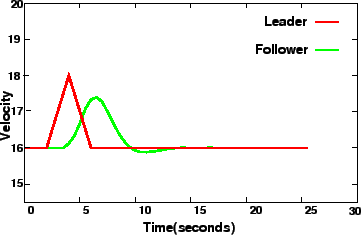 |
Figure 3:
Acceleration vz Time
 |
The earliest car-following models considered the difference in speeds between
the leader and the follower as the stimulus.
It was assumed that every driver tends to move with the same speed as that of
the corresponding leading vehicle so that
 |
(10) |
where is a parameter that sets the time scale of the model and
can be considered as a measure of the sensitivity of the
driver.
According to such models, the driving strategy is to follow the leader and,
therefore, such car-following models are collectively referred to as the follow
the leader model.
Efforts to develop this stimulus function led to five generations of
car-following models, and the most general model is expressed mathematically as
follows.
![\begin{displaymath}
a_{n+1}^{t+{\Delta{T}}}={\frac{\alpha_{l,m} [{v_{n+1}^{t-\De...
...lta{T}}}]^l}}{({v_{n}^{t-\Delta{T}}}-{v_{n+1}^{t-\Delta{T}}})}
\end{displaymath}](img62.png) |
(11) |
where is a distance headway exponent and can take values from +4 to -1,
is a speed exponent and can take values from -2 to +2, and is a
sensitivity coefficient.
These parameters are to be calibrated using field data.
Simulation modeling is an increasingly popular and effective tool for
analyzing a wide variety of dynamical problems which are difficult to be
studied by other means.
Usually, these processes are characterized by the interaction of many system
components or entities.
Traffic simulations models can meet a wide range of requirements:
- Evaluation of alternative treatments
- Testing new designs
- As an element of the design process
- Embed in other tools
- Training personnel
- Safety Analysis
Simulation models are required in the following conditions
- Mathematical treatment of a problem is infeasible or inadequate due to
its temporal or spatial scale
- The accuracy or applicability of the results of a mathematical
formulation is doubtful, because of the assumptions underlying (e.g., a linear
program) or an heuristic procedure (e.g., those in the Highway Capacity Manual)
- The mathematical formulation represents the dynamic traffic/control
environment as a simpler quasi steady state system.
- There is a need to view vehicle animation displays to gain an
understanding of how the system is behaving
- Training personnel
- Congested conditions persist over a significant time.
Simulation models are classified based on many factors like
- Continuity
- Continuous model
- Discrete model
- Level of detail
- Macroscopic models
- Mesoscopic models
- Microscopic models
- Based on Processes
- Deterministic
- Stochastic
Microscopic traffic flow modeling focuses on the minute aspects of traffic
stream like vehicle to vehicle interaction and individual vehicle behavior.
They help to analyze very small changes in the traffic stream over time and
space.
Car following model is one such model where in the stimulus-response concept is
employed.
Optimal models and simulation models were briefly discussed.
- The minimum safe distance headway increases linearly with speed.
Which model follows this assumption?
- Forbe's model
- Pipe's model
- General motor's model
- Optimal velocity model
- The most popular of the car following models is
- Forbe's model
- Pipe's model
- General motor's model
- Optimal velocity model
- The minimum safe distance headway increases linearly with speed.
Which model follows this assumption?
- Forbe's model
- Pipe's model

- General motor's model
- Optimal velocity model
- The most popular of the car following models is
- Forbe's model
- Pipe's model
- General motor's model
- Optimal velocity model
- 1
L J Pignataro.
Traffic Engineering: Theory and practice.
Prentice-Hall, Englewoods Cliffs,N.J., 1973.
Prof. Tom V. Mathew
2011-09-08
![\begin{eqnarray*}
v_n^{t}-v_{n+1}^t = \tau.a_{n+1}^t\\
a^t_{n+1} = \frac{1}{\tau}[v^t_{n}-v^t_{n+1}]
\end{eqnarray*}](img31.png)
$](img44.png)