Macroscopic traffic flow modeling
Lecture notes in Transportation Systems Engineering
3 August 2009
If one looks into traffic flow from a very long distance, the flow of fairly heavy traffic appears like a stream of a fluid.
Therefore, a macroscopic theory of traffic can be developed with the help of hydrodynamic theory of fluids by considering traffic as an effectively one-dimensional compressible fluid.
The behaviour of individual vehicle is ignored and one is concerned only with the behaviour of sizable aggregate of vehicles.
The earliest traffic flow models began by writing the balance equation to address vehicle number conservation on a road.
Infact, all traffic flow models and theories must satisfy the law of conservation of the number of vehicles on the road.
Assuming that the vehicles are flowing from left to right, the continuity equation can be written as
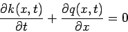 |
(1) |
where  denotes the spatial coordinate in the direction of traffic flow,
  is the time,
  is the density and
  denotes the flow.
However, one cannot get two unknowns, namely
denotes the flow.
However, one cannot get two unknowns, namely  by and
  by solving one equation.
One possible solution is to write two equations from two regimes of the flow, say before and after a bottleneck.
In this system the flow rate before and after will be same, or
by solving one equation.
One possible solution is to write two equations from two regimes of the flow, say before and after a bottleneck.
In this system the flow rate before and after will be same, or
 |
(2) |
From this the shockwave velocity can be derived as
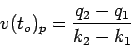 |
(3) |
This is normally referred to as Stock's shockwave formula.
An alternate possibility which Lighthill and Whitham adopted in their landmark study is to assume that the flow rate is determined primarily by the local density , so that flow can be treated as a function of only density .
Therefore the number of unknown variables will be reduced to one.
Essentially this assumption states that k(x,t) and q (x,t) are not independent of each other.
Therefore the continuity equation takes the form
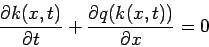 |
(4) |
However, the functional relationship between flow and density cannot be calculated from fluid-dynamical theory.
This has to be either taken as a phenomenological relation derived from the empirical observation or from microscopic theories.
Therefore, the flow rate is a function of the vehicular density k;  .
Thus, the balance equation takes the form
.
Thus, the balance equation takes the form
|
(5) |
Now there is only one independent variable in the balance equation, the vehicle density .
If initial and boundary conditions are known, this can be solved.
Solution to LWR models are kinematic waves moving with velocity
 |
(6) |
This velocity  is positive when the flow rate increases with density, and it is negative when the flow rate decreases with density.
In some cases, this function may shift from one regime to the other, and then a shock is said to be formed.
This shockwave propagate at the velocity
is positive when the flow rate increases with density, and it is negative when the flow rate decreases with density.
In some cases, this function may shift from one regime to the other, and then a shock is said to be formed.
This shockwave propagate at the velocity
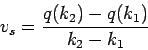 |
(7) |
where  and
and  are the flow rates corresponding to the upstream density
  and downstream density
  of the shockwave.
Unlike Stock's shockwave formula there is only one variable here.
of the shockwave.
Unlike Stock's shockwave formula there is only one variable here.
- 1
D Chowdhury, L Santen, and A Schadschneider.
Statistical physics of vehicular traffic and some related systems.
Physics Report 329, 2000.
199-329.
Prof. Tom V. Mathew
2009-08-03