Cell transmission models

Lecture notes in Transportation Systems Engineering

August 11, 2011

Introduction

In the classical methods to explain macroscopic behaviour of traffic, like hydrodynamic theory, differential equations need to be solved to predict traffic evolution. However in situations of sudden high density variations, like bottlenecking, the hydrodynamic model calls for a shock wave (an ad-hoc). Hence these equations are essentially piecewise continuous which are difficult to solve. Cell transmission models are developed as a discrete analogue of these differential equations in the form of difference equations which are easy to solve and also take care of high density changes. In this lecture note the hydrodynamic model and cell transmission model and their equivalence is discussed. The cell transmission model is explained in two parts, first with only a source and a sink, and then it is extended to a network. In the first part, the concepts of basic flow advancement equations of CTM and a generalized form of CTM are presented. In addition, the phenomenon of instability is also discussed. In the second part, the network representation and topologies are established, after which the model is discussed in terms of a linear program formulation for merging and diverging.

CTM: Single source and a sink

The cell transmission model simulates traffic conditions by proposing to simulate the system with a time-scan strategy where current conditions are updated with every tick of a clock. The road section under consideration is divided into homogeneous sections called cells, numbered from $i$ = 1 to I. The lengths of the sections are set equal to the distances travelled in light traffic by a typical vehicle in one clock tick. Under light traffic condition, all the vehicles in a cell can be assumed to advance to the next with each clock tick. i.e,

$$n_{i+1}(t+1) = n_{i}(t)$$ (1)

where, $n_i(t)$ is the number of vehicles in cell $i$ at time $t$. However equation 1 is not reasonable when flow exceeds the capacity. Hence a more robust set of flow advancement equations are presented next.

Flow advancement equations

First, two constants associated with each cell are defined, namely,$N_i(t)$ and $Q_i(t)$

1. $N_i(t)$ is the maximum number of vehicles that can be present in cell $i$ at time $t$, it is the product of the cell's length and its jam density.
2. $Q_i(t)$ is the maximum number of vehicles that can flow into cell $i$ when the clock advances from $t$ to $t+1$ (time interval $t$), it is the minimum of the capacity of cells from $i-1$ and $i$. It is called the capacity of cell $i$. It represents the maximum flow that can be transferred from $i-1$ to $i$.

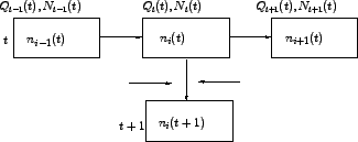
Figure 1: Flow advancement

Now the flow advancement equation can be written as:

$$n_i(t+1) = n_i(t)+y_i(t) - y_{i+1}(t)$$ (2)

where, $n_i(t+1)$ is the cell occupancy at time $t+1$, $n_i(t)$ the cell occupance at time $t$, $y_i(t)$ is the inflow at time $t$, $y_{i+1}(t)$ is the outflow at time $t$. The flows are related to the current conditions at time $t$ as indicated below:

$$y_i(t) = min [n_{i-1}(t), Q_i(t), N_i(t) - n_i(t)]$$ (3)

where, $n_{i-1}(t)$ is the number of vehicles in cell $i-1$ at time $t$, $Q_i(t)$ is the capacity flow into $i$ for time interval $t$, and $N_i(t)$ - $n_i(t)$ is the amount of empty space in cell $i$ at time $t$.

Boundary conditions

Boundary conditions are specified by means of input and output cells. The output cell, a sink for all exiting traffic, should have infinite size ( $N_{I+1} = \infty$) and a suitable, possibly time-varying, capacity. Input cells are a cell pair. A source cell numbered 00 with an infinite number of vehicles ( $n_{00}(O) = \infty$) that discharges into an empty gate cell 00 of infinite size, $N_{0}(t) = \infty$. The inflow capacity $Q_0(t)$ of the gate cell is set equal to the desired link input flow for time interval $t+1$.

Equivalence with Hydrodynamic theory

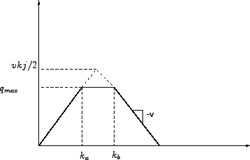
Consider equation 2 and equation 3, they are discrete approximations to the hydrodynamic model with a density- flow (k-q) relationship in the shape of an isoscaled trapezoid, as in Fig.2. This relationship can be expressed as:

$$q = min [v_k, q_{max}, v(k_j - k)], for 0 \leq k \leq k_j,$$ (4)

Flow conservation is given by,

$$\frac{\partial q(x,t)}{\partial x} = \frac{\partial k(x,t)}{\partial t}$$ (5)

To demonstrate the equivalence of the discrete and continuous approaches, the clock tick set to be equal to $\partial t$ and choose the unit of distance such that $v \partial t$ = 1. Then the cell length is 1, $v$ is also 1, and the following equivalences hold: $x \equiv i$, $k_j \equiv N$, $q_{max} \equiv Q$, and $k(x,t) \equiv n_i(t)$ with these conventions, it can be easily seen that the equation 4 & equation 3 are equivalent. Equation 6 can be equivalently written as:

$$y_i(t) - y_{i+1}(t) = - n_i(t)+ n_{i+1}(t+1)$$ (6)

This represents change in flow over space equal to change in occupancy over time. Rearranging terms of this equation we can arrive at equation 3, which is the same as the basic flow advancement equation of the cell transmission model.

Figure 2: Flow-density relationship for the basic cell-transmission model

.

Generalized CTM

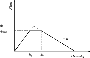
Generalized CTM is an extension of the cell transmission model that would approximate the hydrodynamic model for an equation of state that allows backward waves with speed $w \leq v$ (see Fig. 3 ). This is a realistic model, since on many occassions speed of backward wave will not be same as the free flow speed.

Figure 3: Flow-density relationship for the generalized CTM

$$y_i(t) = min [n_{i-1}(t), Q_i(t), w/v[ N_i(t) - n_i(t)]]$$ (7)

A small modification is made in the above equation to avoid the error caused due to numerical spreading. Equation 7 is rewritten as

$$y_i(t) = min [n_{i-1}(t), Q_i(t),\alpha[Ni_(t) - n_i(t)]]$$ (8)

where,

Numerical example 1

Consider a 1.25 km homogeneous road with v = 50 kmph, kj = 180 vpkm and qmax = 3000 vph. Initially traffic is flowing undisturbed at 80% of capacity: q = 2400 VPH. Then, a partial lane blockage lasting 2 min occurs one third of the distance from the end of the road. The blockage effectively restricts flow to 20% of the maximum. Clearly, a queue is going to build and dissipate behind the restriction. Predict the evolution of the traffic. Take one clock tick as 30 seconds.

Solution :

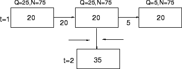
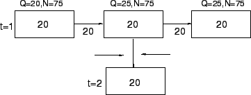
Initialization of the table: Choosing clock tick as 30seconds.(i.e1/120th of an hr.) Cell length=50/120=5/12th of a km. Number of cells=1.25*12/5=3. Cell constants: N= 180*5/12=75 Q=3000/120=25. 2min=120s=4 clock ticks. Initial occupancy=2400/120=20. Table at the start of the simulation. (see Fig. ) Note: Simulation need not be started in any specific order, it can be started from any cell in the row corresponding to the current clock tick. For illustration, consider cell 2 at time 2 in the final table (see Fig.), its entry depends on the cells marked with rectangles. By flow conservation law: Occupancy = Storage + Inflow-Outflow Here, Storage = 20. For inflow use equation 3 Inflow= min [20,min(25,25),(75-20)]= 20 Outflow= min [20,min(25,5),(75-20)]= 5 Occupancy= 20+20-5=35.

For cell 1 at time 2, Inflow= min [20,min(25,25),(75-20)]= 20 Outflow= min [20,min(25,25),(75-20)]= 20 Occupancy= 20+20-20=20.

For cell 3 at time 2, Inflow= min [20, min (25,5),(75-20)]= 5 Outflow= 20 (:.sink cell takes all the vehicles in previous cell) Occupancy= 20+5-20=5.

Numerical example 2

Consider a 1.25 km homogeneous road with v = 50 kmph, kj = 180 vpkm and $q_{max}$ = 3000 vph. Initially traffic is flowing undisturbed at 80% of capacity: q = 2400 VPH. Then, a partial lane blockage lasting 2 min occurs l/3 of the distance from the end of the road. The blockage effectively restricts flow to 20% of the maximum. Clearly, a queue is going to build and dissipate behind the restriction. Predict the evolution of the traffic. Take one clock tick as 6 seconds. Solution: This problem is same as the earlier problem, only change being the clock tick. The simulation is done for this smaller clock tick; the results are shown in Fig.  One can clearly observe the pattern in which the cells are getting updated. After the decrease in capacity on last one-third segment queuing is slowly building up and the backward wave can be appreciated through the first arrow. The second arrow shows the dissipation of queue and one can see that queue builds up at a faster than it dissipates. This simple illustration shows how CTM mimics the traffic conditions.

CTM: Network Traffic

General

As sequel to his first paper on CTM, Daganzo (1995) published first paper on CTM applied to network traffic. In this section application of CTM to network traffic considering merging and diverging is discussed. Some basic notations: (The notations used from here on, are adopted from Ziliaskopoulos (2000)) $\Gamma^{-1}$ = Set of predecessor cells. $\Gamma$ = Set of successor cells.

Network topologies

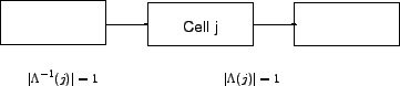
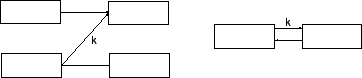
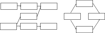
The notations introduced in previous section are applied to different types of cells, as shown in Fig. 4 Some valid and invalid representations in a network are shown in Fig 6.

Figure 4: Source Cell

Figure 5: Sink Cell

Figure 6: Ordinary Cell

Figure 7: Merging Cell

Figure 8: Diverging Cell

Figure 9: Invalid representations

Figure 10: Valid representations

Ordinary link

Consider an ordinary link with a beginning cell and ending cell, which gives the flow between two cells is simplified as explained below.

Figure 11: Ordinary Link

$$y_k(t) = min(n_{Bk}(t), min[Q_{Bk}(t), Q_{Ek}(t)], \delta_{Ek}[ NEk(t) - nEk(t)])$$ (9)

$$S_I(t) = min (QI,nI)$$ (10)

$$R_I(t) = min (Q_I,\delta_I,[N_I- n_I])$$ (11)

$$y_k(t) = min(S_{Bk},R_{Ek})$$ (12)

From equations one can see that a simplification is done by splitting $y_k(t)$ in to $S_{Bk}$ and $R_{Ek}$ terms. 'S' represents sending capacity and 'R' represents receiving capacity. During time periods when $S_{Bk} < R_{Ek}$ the flow on link k is dictated by upstream traffic conditions-as would be predicted from the forward moving characteristics of the Hydrodynamic model. Conversely, when $S_{Bk} > R_{Ek}$, flow is dictated by downstream conditions and backward moving characteristics.

Merging and diverging

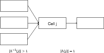
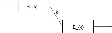
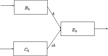
Consider two cells merging, here we have a beginning cell and its complimentary merging into ending cell, the constraints on the flow that can be sent and received are given by equation 15 and equation 15.

$$y_k(t) \leq S_{Bk}$$ (13)

$$y_{ck}(t) \leq S_{Ck}$$ (14)

$$y_k(t)+y_{ck}(t) \leq R_{Ek}$$ (15)

where, $S_I(t)$ is the min $(Q_I,n_I)$, and $R_I(t)$ is the min $(Q_I,\delta I,[N_I- n_I])$.

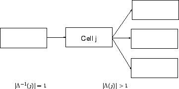
A number of combinations of $y_k(t) +y_{ck}(t)$ are possible satisfying the above said constraints. Similarly for diverging a number of possible outflows to different links is possible satisfying corresponding constraints, hence this calls for an optimization problem. Ziliaskopoulos (2000), has given this LP formulations for both merging and diverging, this has been discussed later

Conclusion

Summary

• CTM is a discrete approximation of hydrodynamic model. System evolution is based on difference equations.
• Unlike hydrodynamic model, it explains the phenomenon of Instability.
• Lesser the time per clock tick lesser are the size of cells and more accurate results would be obtained. But a compromise is needed between accuracy and computational effort. Largest possible cell size which would sufficiently give the details needed must be chosen.
• CTM has many applications in DTA, NDP, traffic operations, emergency evacuations etc.
• There is a vast scope for improvement and applications of this model.

Advantages and applications

• CTM is consistent with hydrodynamic theory, which is a widely used model for studying macroscopic behavior of the traffic.
• It is simple and sufficiently accurate for planning purposes.
• Here two efficient modeling approaches are used, one is Linear Programming, whose characteristics well known and the other is Parallel computing.These are important from the perspective of computational speed and efficiency.
• CTM can be used to provide "real time" information to the drivers.
• CTM has been used in developing a system optimal signal optimization formulation.
• CTM based Dynamic Traffic Assignment have shown good results.
• CTM has its application in Network Design Problems.(NDP)
• Dynamic network models based on CTM can also be applied to evaluate the performance of emergency evacuation plans.

Limitations

• CTM is for a "typical vehicle" in network traffic, work is needed for the multi-modal representation of traffic.
• Cell length cannot be varied. Change in the model has to be brought without loss of generality, to relax the constraint on arbitrary selection of cell length, which will facilitate the modelers to select variable cell lengths that are best aligned with the geometry.
• CTM is largely deterministic, stochastic variables are needed to be introduced to represent the random human behavior.
• Mesoscopic features can be introduced so that concepts like lane changing behavior etc. can be studied.

Bibliography