Congestion Studies
Lecture notes in Transportation Systems Engineering
July 28, 2011
Transportation system consists of a group of activities as
well as entities interacting with each other to achieve the
goal of transporting people or goods from one place to
another.
Hence, the system has to meet the perceived social and
economical needs of the users.
As these needs change, the transportation system itself
evolves and problems occur as it becomes inadequate to serve
the public interest.
One of the negative impacts of any transportation system is
traffic congestion.
Traffic congestion occurs wherever demand exceeds the
capacity of the transportation system.
This lecture gives an overview of how congestion is
generated, how it can be measured or quantified, and also
the various countermeasures to be taken in order to
counteract congestion.
Adequate performance measures are needed in order to
quantify congestion in a transportation system.
Quality of service measures indicates the degree of
traveller satisfaction with system performance and this is
covered under traveller perception.
Several measures have been taken in order to counteract
congestion.
They are basically classified into supply and demand
measures.
An overview of all these aspects of congestion is dealt with
in this lecture.
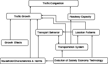
The flow chart in Fig. 1 shows how
traffic congestion is generated in a transportation system.
With the evolution of society, economy and technology, the
household characteristics as well as the transportation
system gets affected.
The change in transport system causes a change in transport
behaviour and locational pattern of the system.
The change in household characteristics, transport
behaviour, locational pattern, and other growth effects
result in the growth of traffic.
But the change or improvement in road capacity is only as
the result of change in the transportation system and hence
finally a situation arises where the traffic demand is
greater than the capacity of the roadway.
This situation is called traffic congestion.
Figure 1:
Generation of traffic congestion
 |
Congestion has a large number of ill effects which include:
- Loss of productive time,
- Increase in the fuel consumption,
- Increase in pollutants (because of both the additional
fuel burned and more toxic gases produced while internal
combustion engines are in idle or in stop-and-go traffic),
- Increase in wear and tear of automobile engines,
- High potential for traffic accidents,
- Negative impact on people's psychological state, which
may affect productivity at work and personal relationships,
and
- Slow and inefficient emergency response and delivery
services.
The summation of all these effects yields a considerable
loss for the society and the economy of an urban area
A system is said to be congested when the demand exceeds the
capacity of the section.
Traffic congestion can be defined in the following two ways:
- Congestion is the travel time or delay in excess of
that normally incurred under light or free flow traffic
condition.
- Unacceptable congestion is travel time or delay in
excess of agreed norm which may vary by type of transport
facility, travel mode, geographical location, and time of
the day.
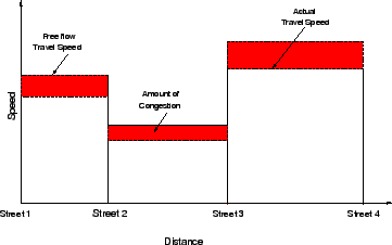
Fig. 2 shows the definition of congestion.
The solid line represents the travel speed under free-flow
conditions and the dotted line represents the actual travel
speed.
During congestion, the vehicles will be travelling at a
speed less than their free flow speed.
The shaded area in between these two lines represents the
amount of congestion.
Figure 2:
Definition of congestion
 |
Traffic congestion may be of two types:
- Recurrent Congestion: Recurrent congestion
generally occurs at the same place, at the same time every
weekday or weekend day.
- Non-Recurrent congestion: Non-Recurrent
congestion results from incidents such as accidents or
roadway maintenance.
Congestion has to be measured or quantified in order to
suggest suitable counter measures and their evaluation.
Congestion information can be used in a variety of policy,
planning and operational situations.
It may be used by public agencies in assessing facility or
system adequacy, identifying problems, calibrating models,
developing and assessing improvements, formulating programs
and policies and priorities.
It may be used by private sector in making locational or
investment decisions.
It may be used by general public and media in assessing
traveller's satisfaction.
Performance measure of a congested roadway can be done using
the following four components:
- Duration,
- Extent,
- Intensity, and
- Reliability.
Duration of congestion is the amount of time the congestion
affects the travel system.
The peak hour has now extended to peak period in many
corridors.
Measures that can quantify congestion include:
- Amount of time during the day that the travel rate
indicates congested travel on a system element or entire
system.
- Amount of time during the day that traffic density
measurement techniques (detectors, aerial surveillance,
etc.) indicate congested travel.
Duration of congestion is the sum of length of each analysis
sub period for which the demand exceeds capacity.
The maximum duration on any link indicates the amount of
time before congestion is completely cleared from the
corridor.
Duration of congestion can be computed for a corridor using
the following equation:
 |
(1) |
where,  is the duration of congestion (hour),
  is the
number of analysis sub periods for which
is the
number of analysis sub periods for which  , and
, and
 is the duration of analysis sub-period (hour)The
duration of congestion for an area is given by:
is the duration of analysis sub-period (hour)The
duration of congestion for an area is given by:
 |
(2) |
where,
 is the duration of congestion for link
  (hour),
is the duration of analysis period (hour),
(hour),
is the duration of analysis period (hour),
 is the ratio of peak demand to peak demand rate,
 is the vehicle demand on link (veh/hour), and
 is the capacity of link (veh/hour).
Extent of congestion is described by estimating the number
of people or vehicles affected by congestion and by the
geographic distribution of congestion.
These measures include:
is the capacity of link (veh/hour).
Extent of congestion is described by estimating the number
of people or vehicles affected by congestion and by the
geographic distribution of congestion.
These measures include:
- Number or percentage of trips affected by congestion.
- Number or percentage of person or vehicle meters
affected by congestion.
- Percentage of the system affected by congestion.
Performance measures of extent of congestion can be computed
from sum of length of queuing on each segment.
Segments in which queue overflows the capacity are also
identified.
To compute queue length, average density of vehicles in a
queue need to be known.
The default values suggested by HCM 2000 are given in Table
1.
Table 1:
Queue density default values
| Subsystem |
Storage density(veh/km/lane) |
Spacing(m) |
| Free-way |
75 |
13.3 |
| ]
Two lane highway |
130 |
7.5 |
| Urban street |
130 |
7.5 |
Queue length can be found out using the equation:
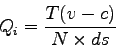 |
(3) |
where;
 is the queue length (meter),
 is the segment demand (veh/hour),
 is the segment capacity (veh/hour),
is the number of lanes,
is the segment capacity (veh/hour),
is the number of lanes,
 is the storage density (veh/meter/lane), and
is the duration of analysis period (hour).
If
is the storage density (veh/meter/lane), and
is the duration of analysis period (hour).
If  , =0 The equation for queue length is similar
for both corridor and area-wide analysis.
Intensity of congestion marks the severity of congestion.
It is used to differentiate between levels of congestion on
transport system and to define total amount of congestion.
It is measured in terms of:
, =0 The equation for queue length is similar
for both corridor and area-wide analysis.
Intensity of congestion marks the severity of congestion.
It is used to differentiate between levels of congestion on
transport system and to define total amount of congestion.
It is measured in terms of:
- Delay in person hours or vehicle hours;
- Average speed of roadway, corridor, or network;
- Delay per capita or per vehicle travelling in the
corridor, or per person or per vehicle affected by
congestion;
- Relative delay rate (relative rate of time lost for
vehicles);
Intensity in terms of delay is given by,
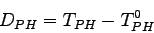 |
(4) |
where,
 is the person hours of delay,
 is the person hours of travel under actual
conditions, and
is the person hours of travel under actual
conditions, and
 is the person hours of travel under free flow
conditions.
The is given by:
is the person hours of travel under free flow
conditions.
The is given by:
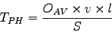 |
(5) |
where,
 is the average vehicle occupancy,
is the vehicle demand (veh),
is the average vehicle occupancy,
is the vehicle demand (veh),
 is the length of link (km), and
 is the mean speed of link (km/h). The is given
by:
is the mean speed of link (km/h). The is given
by:
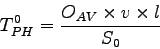 |
(6) |
where,
is the average vehicle occupancy,
is the vehicle demand (veh),
is the length of link (km), and
 is the free flow speed on the link
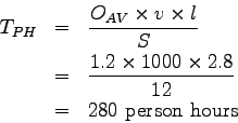
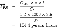
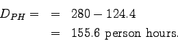
On a 2.8 km long link of road, it was found that the demand
is 1000 Vehicles/hour mean speed of the link is 12 km/hr,
and the free flow speed is 27 km/hr.
Assuming that the average vehicle occupancy is 1.2
person/vehicle, calculate the congestion intensity in terms
of total person hours of delay.
Person hours of delay is given as
is the free flow speed on the link
On a 2.8 km long link of road, it was found that the demand
is 1000 Vehicles/hour mean speed of the link is 12 km/hr,
and the free flow speed is 27 km/hr.
Assuming that the average vehicle occupancy is 1.2
person/vehicle, calculate the congestion intensity in terms
of total person hours of delay.
Person hours of delay is given as
Person hours of travel under actual conditions,
Person hours of travel under free flow conditions,
Therefore, person hours of delay,
The relationship between duration,extent, and intensity of
congestion can be show in a time-distance graph
Fig. 3
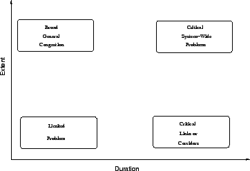
The extent of congestion is seen on the x-axis, the duration
on the y-axis. The intensity is shown in the shading. Based
on the extent and duration the congestion can be classified
into four types as shown in Fig.4
Figure 3:
Intensity of congestion-relation between duration
and distance
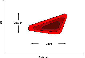 |
The variation in extent and duration of congestion indicates
different problems requiring different solutions.
Small delay and extent indicates limited problem, small
delay for large extent indicates general congestion, great
delay for small extent indicates critical links and great
delay for large extent indicates critical system-wide
problem.
Figure 4:
Intensity of congestion-Relation between extent and
duration of delay
 |
The product of extent and duration indicates the intensity,
or magnitude of the congestion problem.
Various measures to address congestion are discussed here.
These include supply side, demand side, and pricing.
Congestion countermeasures on the supply side add capacity
to the system or make the system operate more efficiently.
They focus on the transportation system. Supply measures
include
- Development of new or expanded infrastructure.
This includes civil projects (new freeways, transit lines
etc), road widening, bridge replacement, technology
conversions(ITS),etc.
- Small scale capacity and efficiency improvement.
This includes signal system upgrade and coordination,
freeway ramp metering, re-location of bus stops etc.
Demand measures focuses on motorists and travelers and
attempt to modify their trip making behaviour.
Demand measures include:
- Parking pricing:
It discourages the use of private vehicles to specific
areas, thereby reducing the demand on the transportation
system.
- Restrictions on vehicle ownership and use: It includes
heavy import duties, separate licensing requirement, heavy
annual fees, expensive fuel prices, etc. to restrain private
vehicle acquisition and use.
Congestion pricing is a method of road user taxation,
charging the users of congested roads according to the time
spent or distance travelled on them.
The principle behind congestion pricing is that those who
cause congestion or use road in congested period should be
charged, thus giving the road user the choice to make a
journey or not.
Journey costs are made of private journey cost, congestion
cost, environmental cost, and road maintenance cost.
The benefit a road user obtains from the journey is the
price he prepared to pay in order to make the journey.
As the price gradually increases, a point will be reached
when the trip maker considers it not worth performing or
worth performing by other means.
This is known as the critical price. At a cost less than
this critical price, he enjoys a net benefit called as
consumer surplus(es) and is given by:
 |
(7) |
where,
 is the amount the consumer is prepared to pay, and
 is the amount he actually pays.
The basics of congestion pricing involves demand function,
private cost function as well as marginal cost function.
These are explained below.
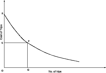
Fig. 5 shows the general form of a demand
curve.
In the figure, area QOSP indicates the absolute utility to
trip maker and the area SRP indicates the net benefit.
is the amount he actually pays.
The basics of congestion pricing involves demand function,
private cost function as well as marginal cost function.
These are explained below.
Fig. 5 shows the general form of a demand
curve.
In the figure, area QOSP indicates the absolute utility to
trip maker and the area SRP indicates the net benefit.
Figure 5:
Demand Curve
 |
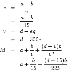
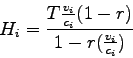
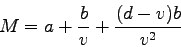
Total private cost of a trip, is given by:
 |
(8) |
where,
 is the component proportional to distance,
 is the component proportional to speed, and
is the speed of the vehicle (km/h) which is given by:
is the component proportional to speed, and
is the speed of the vehicle (km/h) which is given by:
 |
(9) |
where,
 is the flow in veh/hour,
 and e are constants.
Marginal cost is the additional cost of adding one extra
vehicle to the traffic stream. It reduces speed and causes
congestion and results in increase in cost of all journey.
The total cost incurred by all vehicles in one hour(
and e are constants.
Marginal cost is the additional cost of adding one extra
vehicle to the traffic stream. It reduces speed and causes
congestion and results in increase in cost of all journey.
The total cost incurred by all vehicles in one hour( )
is given by:
)
is given by:
 |
(10) |
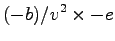
Marginal cost is obtained by differentiating the total cost
with respect to the flow() as shown in the following
equations.
 |
 |
 |
(11) |
 |
|
 |
(12) |
| |
|
 |
(13) |
| |
|
 |
(14) |
|
|
|
(15) |
| |
|
 |
(16) |
Note that c and q in the above derivation is obtained from
Equations 8 and 9 respectively.
Therefore the marginal cost is given as:
 |
(17) |
Fig. 6 shows the variation of marginal cost
per flow as well as private cost per flow.
Figure 6:
Private cost/flow and cost and marginal curve
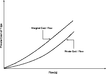 |
It is seen that the marginal cost will always be greater
than the private cost, the increase representing the
congestion cost.
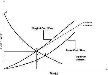
Superimposing the demand curve on the private cost/flow and
marginal cost/flow curves, the position as shown in
Fig. 7 is obtained.
The intersection of the demand curve and the private costs
curve at point A represents the equilibrium condition,
obtained when travel decisions are based on private costs
only.
The intersection of the demand curve and the marginal costs
curve at point B represents the optimum condition.
The net benefit under the two positions A and B are shown by
the areas ACZ and  respectively. If the conditions
are shifted from point A to B, the net benefit due to change
will be given by area
respectively. If the conditions
are shifted from point A to B, the net benefit due to change
will be given by area  minus AXB.
If the area is greater than arc AXB, the net
benefit will be positive.
The shifting of conditions from point A to B can be brought
about by imposing a road pricing charge BY.
Under this scheme, the private vehicles continuing to use
the roads will on an average be worse off in the first place
because BY will always exceed the individual increase in
benefits XY.
minus AXB.
If the area is greater than arc AXB, the net
benefit will be positive.
The shifting of conditions from point A to B can be brought
about by imposing a road pricing charge BY.
Under this scheme, the private vehicles continuing to use
the roads will on an average be worse off in the first place
because BY will always exceed the individual increase in
benefits XY.
Figure 7:
Relation between material cost, private cost and
demand curves.
 |
Vehicles are moving on a road at the rate of 500
vehicle/hour, at a velocity of 15 km/hr. Find the equation
for marginal cost.
- Diverts travelers to other modes
- Causes cancellation of non essential trips during peak
hours
- Collects sufficient fund for major upgrades of
highways
- Cross-subsidizes public transport modes
- Charges should be closely related to the amount of use
made of roads
- Price should be variable at different times of
day/week/year or for different classes of vehicles
- It should be stable and ascertainable by road users
before commencement of journey
- Method should be simple for road users to understand
and police to enforce
- Should be accepted by public as fair to all
- Payment in advance should be possible
- Should be reliable
- Should be free from fraud or evasion
- Should be capable of being applied to the whole
country
In this lecture, we have discussed about the causes and
effects of congestion and how congestion can be defined.
We also discussed how congestion can be quantified by
various performance measures such as
duration, extent and intensity.
The measures to be taken in order to counteract congestion
were also discussed.
The principle and process of congestion pricing was also
discussed.
Prof. Tom V. Mathew
2011-07-28