Problem 5.1.: The table below shows the data from a spot speed study. Find the PCUvalue of each vehicle type using Chandra's Method. (Use the table from the notes to get the projected area of each vehicle type. All the speeds are in meters/sec.)
| No | Car | 3W | 2W | Cycle | LCV | HCV |
| 1 | 11.32 | 8.67 | 6.67 | 4.1 | 6.0 | 7.4 |
| 2 | 6.74 | 7.25 | 8.27 | 7.57 | 6.88 | 6.09 |
| 3 | 11.11 | 9.68 | 7.75 | 5.66 | 7.5 | 5.88 |
| 4 | 6.67 | 6.98 | 6.12 | 3.4 | 8.57 | 6.38 |
| 5 | 8.11 | 8.77 | 9.52 | 4.11 | 9.67 | 5.66 |
| 6 | 7.41 | 8.77 | 11.9 | 2.65 | 8.57 | 5.66 |
| 7 | 8.11 | 9.52 | 6.97 | 4.28 | 5.7 | 5.55 |
| 8 | 9.93 | 9.4 | 6.97 | 4.19 | 4.68 | 6.12 |
| 9 | 6.25 | 8.12 | 9.09 | 5.89 | 5.69 | 5.2 |
| 10 | 5.29 | 9.68 | 7.69 | 6.0 | 7.21 | 5.54 |
| 11 | 8.33 | 7.75 | 5.7 | 5.9 | 5.74 | 8.67 |
| 12 | 8.57 | 8.33 | 9.09 | 3.79 | 6.53 | 3.1 |
| 13 | 9.34 | 5.51 | 8.33 | 3.92 | 7.24 | 4.61 |
| 14 | 7.24 | 5.17 | 5.45 | 4.11 | 5.66 | 3.95 |
| 15 | 8.11 | 5.0 | 7.89 | 3.18 | 5.42 | 4.68 |
| 16 | 10 | 8.33 | 6.52 | 4.98 | 4.97 | 4.1 |
| 17 | 7.58 | 5.55 | 9.8 | 4.48 | 5.76 | 5.56 |
| 18 | 11.11 | 8.33 | 9.14 | 2.96 | 6.12 | 4.76 |
| 19 | 7.09 | 7.5 | 7.14 | 4.87 | 6.38 | 5.6 |
| 20 | 4.02 | 5.25 | 6.97 | 4.1 | 4.83 | 4.61 |
Problem 6.1:
For the following spot speed data (in kmph) collected from a freeway site operating
under free-flow conditions: (i) Plot the frequency and cumulative frequency
curves for these data. (ii) Find and identify on the curves: median speed,
modal speed, pace, percent vehicles in pace, quartile speeds and percentile
speeds (15, 85, & 98). (iii) Compute the mean and standard deviation of the
speed distribution. (iv) Based on the results obtained, determine the
confidence level of study if error ±1.8 km/h is allowed for sample data
collected? (v) What are the confidence bounds on the estimate of the true mean
speed of the underlying distribution with 95% confidence? With 99.7%
confidence?
| Speed Range | Frequency |
| 26 - 30 | 6 |
| 31 - 35 | 13 |
| 36 - 40 | 26 |
| 41 - 45 | 33 |
| 46 - 50 | 27 |
| 51 - 55 | 25 |
| 56 - 60 | 24 |
| 61 - 65 | 20 |
| 66 - 70 | 17 |
| 71 - 75 | 12 |
| 76 - 80 | 8 |
| 81 - 85 | 5 |
Problem 7.1: A test was conducted to determine the delay in an intersection. The table below presents the observed vehicle-in-queue counts at the intersection. The traffic signal at the intersection operates with a cycle time of 140sec. The test was conducted on the 2 lane road over a 30-min period, which is almost thirteen cycles .Count interval was 15-s. The total number of stopped vehicle and not-stopped vehicle are 190 and 80 respectively. Calculate the control delay per vehicle of the road using HCM 2000 method. Assume the free flow speed to be 65 km/h and the empirical adjustment factor 0.9
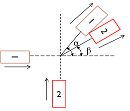
Problem 15.1: For the given state of traffic predict if the subject vehicle in the figure would initiate a lane change. If yes what is the feasibility and probability of lane change. Given is the mid block section of 2 lane highway with no other blocks in either of the lane. Neglect lateral acceleration. Consider update time 1 sec. Maximum deceleration driver ready to apply is -2 m/s2 and maximum deceleration feasible is -2.2 m/s2 .consider the gap between front of the subject vehicle and the rear of preceding vehicle to be 160 m. Use GIPPS model of lane change. Refer the figure given below.
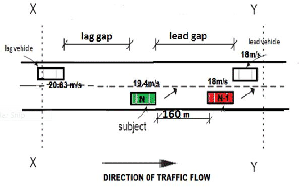
Problem 15.2: For the same speed of all the four vehicles what is the feasibility of the lane change (assuming the trigger has already occurred). Lag gap available at the time of trigger is 15 s and Lead gap is 40 s. Assume the vehicle take 1s to shift the lane laterally.
Problem 15.3:
Under the state traffic given in question 1 what is the probability of gap
acceptance by the driver. Given ![]() =2 ,
=2 , ![]() = 3,
= 3, ![]() =40m,
=40m, ![]() =50m,
=50m,
 =
=  = 1,
= 1,
 = 0.8,
 = 0.7,
![]() = 1.2.
= 1.2.
Problem 16.1:
The parameters obtained in GM car-following model simulation are given in the
following table. Field observed values of acceleration of follower is also
given. Calibrate the model by finding the value of ![]() . Assume l=1 and m=0.
Formulate as an optimization problem and solve it analytically.
. Assume l=1 and m=0.
Formulate as an optimization problem and solve it analytically.
| dv | dx | |
| 0.23 | 1.5 | 29.13 |
| 0.46 | 1.88 | 29.97 |
| 0.67 | 1.16 | 30.73 |
| 0.82 | 0.32 | 31.10 |
Problem 16.2: The observed and simulated values obtained using Model 1 and Model 2 are given in the table below. (i) Comment on the performance of both the models based on the following error measures - Root Mean Square Error, Root Mean Squared Normalized Error, Mean Error and Mean Normalized Error. (ii) Using Theil's indicator, comment on the acceptability of the models.
| Observed | Model 1 | Model 2 |
| 0.23 | 0.2 | 0.27 |
| 0.46 | 0.39 | 0.5 |
| 0.67 | 0.71 | 0.65 |
| 0.82 | 0.83 | 0.84 |
Problem 18.1: Consider a 1 km homogeneous road with speed (v) 60 kmph, jam density (kj) 180 veh/km, and maximum flow (qmax) 3000 veh/hr. Initially traffic is flowing undisturbed at 80% of capacity (q) which is 2400 veh/hr. Then, a partial lane blockage lasting 3 min occurs on l/3rd of the distance from the end of the road. The blockage effectively restricts flow to 20% of the maximum. Clearly, a queue is going to build and dissipate behind the restriction. After 3 minutes, the flow in cell 3 is maximum possible flow. Predict the evolution of the traffic. Take one clock tick as 20 seconds.
Problem 20.1: Assume a single lane road stretch divided into 9 cells and vehicles are present in the first, fourth, seventh and eight cells with 3, 2, 0, 1 as their velocities respectively. Apply the rules of CA and update the position of the vehicles for the next three second. Assume suitable randomization probability.
Problem 20.2: Assume a two-lane road divided into nine cells in each of its lane. In first lane vehicles are present in first (1), third (0), fourth (1), eight (1) cells and in second lane vehicles are present in fifth (1) and sixth (0) cells. The numbers in the brackets indicate the present velocities of the respective velocities. Apply the lane changing rules and determine which vehicles fulfilled the lane changing requirements.
Problem 19.1: The flows from an upstream point to a downstream point which is 390m away are given. Calculate the downstream flows, assuming the model time step duration as 10sec. The average speed of the vehicles can be taken as 40kmph. Upstream flows: q (at 10sec) =25, q (at 20 sec) =18, q (at 30 sec) =21, q (at 40 sec) =27, and q (at 50 sec) = 20. The standard deviation for travel time is 8.
Problem 22.1: Given the total number of stopped vehicles is 1589 and number of exiting vehicles is 832, calculate the approach delay for the intersection. Consider sampling interval as 15sec. Also, determine LOS if FFS of urban street is 70 kmph, segment length is 1200m.
Problem 23.1: A 8 km long 6 lane divided multilane highway in a suburban area has a segment 2 km long with a 3% upgrade and a segment 1 km long with a 2% downgrade. The section has a volume of 1500 vehicles/hr in each direction with 13% trucks and buses and no recreational vehicles has field measured FFS of 75 km/hr on upgrade and 80 km/hr on downgrade. There are total of 6 access points/km WB and 4 access points/km EB on the upgrade stretch and 4 access points/km WB and 5 access points/km EB on the downgrade stretch. The lane width is 3.6 m, PHF is 0.90 and having a 3.6 m lateral clearance. Determine the LOS of the highway section (upgrade and downgrade) during the peak hour? From HCM, For a 3% upgrade and 2 km length (ET=2) For a 2% downgrade and 1 km length (ET=1.5)
Problem 24.1: Consider an existing six lane freeway in urban area, having very restricted geometry with level terrain. Peak hour volume is 2400 veh/h with 5 % trucks. The traffic is commuter type with peak hour factor 0.88 and interchange density as 0.9 interchanges per kilometer. Freeway consists of 3 lanes in each direction of 3.6 m width with lateral clearance of 1.2 m. Find the LOS of freeway during peak hour.
Problem 25.1: Consider an on-ramp and an off-ramp, both single lane, to an eight lane freeway. The length of both the acceleration lane and the deceleration lane is 80 m. During peak hour find: (i) LOS of merge area for on-ramp (Given: Peak hour factor=0.9, freeway volume is 5500 vph, on ramp volume is 400 vph,driver adjustment factor is 1.0, heavy vehicle adjustment factor for freeway is 0.952 and for ramp is 0.976 and proportion of freeway vehicles in lanes 1 and 2 is 25.5%); (ii) LOS of diverge area for off-ramp . (Given: Peak hour factor=0.9, off ramp volume is 600 vph, driver adjustment factor is 1.0, heavy vehicle adjustment factor for freeway is 0.954 and for ramp is 0.952 and proportion of freeway vehicles in lanes 1 and 2 is 43.6%). Assume suitable data if necessary.
Problem 26.1: Consider the geometry given below in Fig. 2 shows the urban subsystem network all intersections are Signalized, all arterial are two directional and the necessary inputs are also given as below Find the performance measurement of the subsystem. The number of lane for all urban streets is 2 for each direction; AVO=1.2. There is no any bicycle and pedestrian traffic on the system.
Peak Hour Demand data all Volumes are in (veh/hr) is given in the Table 2 (Note that NL, NT, NR refers to the north bound left, through, and right traffic). Capacities, Lengths, Free flow speeds and average flow speeds for each link input data is also given in the Table 3.
|
Problem 31.1: Provide channelization for an T intersection near YP Gate IIT Campus, having NS as major road (Canara Bank to YP) intersect at right angle. Design vehicle is SU (single unit truck) and design speed is 30 kmph take (R=25). `The intersection is signalized. NS road has 2 lanes in each direction and EW has 1 lane for each direction. Take lane width 3.6m. provide a suitable median along with island for free left turn EN and SW bound traffic.
Problem 35.1: Consider the following situation: An intersection approach has an approach flow rate of 1750 vph, a saturation flow rate of 2500 vphg, a cycle length of 90 s, and effective green ratio for the approach 0.55. Assume Progression Adjustment Factor 1.2 and delay due to pre-existing queue, 42 sec/veh .What control delay sec per vehicle is expected under these conditions?
Problem 36.1: If there is 30 percent right turning movement, and through-car equivalent for permitted right turns is 3, saturation headway is 2 sec; ideal saturation flow is 1800. Find the value of Adjusted Saturation flow.
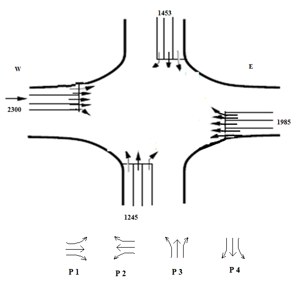
Problem 36.2: Find Critical Volume (Vi) for a four arm Intersection. Traffic flow Proportion of Left and Right turn are 10(For all approach). Left and Right turn Lane utilization factors are 0.2 and 0.3 respectively. The geometry and the phase palan is given in the figure.
Problem 37.1: Calculate capacity and levele of service for WB, NB and SB approach individually and the the level of service of the signalized intersection for the first example of the HCM 2000 chapter 16. Provide detailed calculation.
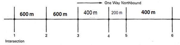
Problem 38.1: Consider the one-way arterial shown in figure 3, with the link lengths indicated. If the platoon speed is 20 m/s. and The cycle length is 60 s, and the effective green time at each intersection is 50lane, discharge headway 2 sec and start-up lost time, 2s. Find the band width with Time space diagram? `
Problem 39.1: Consider an intersection of two streets with 2 lanes in each direction. Each approach has flow rate 800 veh/hr with no left or right turns. The lost time per phase is 3 secs and the length of detectors is 9.1 m with no setback from the stop line. The average headway is 1.8 secs and the actuated controller settings are as follows: Initial interval is 12 sec, the unit extension is 3 sec, the maximum green time is 45 sec, and the intergreen time is 4 sec. Determine the phase time for this intersection considering an approach speed of 50 kmph.
Problem 40.1: Compare and contrast the working principle of SCAT and SCOOT modelswith the help of typical sketches.
Problem 40.2: What are the challenges in implementing ATC in India?
Problem 41.1: Two vehicles are approaching at right angles, the first from west and the second from the south, collide with each other (refer figure 5). After the collision, the first vehicle skids in a direction 60 degrees east of north and the second vehicle skids in a direction of 30 degrees east of north. Initial skid distance of the first and second vehicles are 48 and 30 meters respectively before collision and skid distance after collision are 25 and 46 meters respectively. If the weights of the first and second vehicles are 7.0 and 5.5 tonnes respectively, calculate the original speed of vehicles. The average skid resistance of pavement is found to be 0.5.
Problem 43.1: A city has a total of 120000 commuters traveling at an average speed of 30 kmph, and using an arterial road of length 30 km. Due to the congestion and parking problems, 30% commuters form car pools with a car occupancy of 3.0 and 30% arrange for subscription bus service (60 seater). Rest of the commuters choose to travel by private cars. The peak period congestion was found to be reduced and the speed was increased to 40 kmph. Assuming the no. of stops to be 9, calculate the amount of fuel saved. i(Assume k1 = 0.075 liters/km, k2 = 1.75 liters/hr.
Problem 43.2: Calculate the total fuel consumption by a vehicle traveling on a stretch of road of length 20 km. The average stopped delay for the vehicle is 5 sec. The vehicle stops 5 times during its journey. Assume f1, f2, and f3 as 0.005, 0.0045, and 0.003 respectively.
Problem 44.1: Consider a road segment of 4 lanes with a capacity of 2465 veh/hr/lane. It is observed that the storage density is 130 veh/meter and the segment demand is found to be 3000 veh/hr/lane. Given that the duration of analysis sub period is 3 hrs calculate the queue length that is formed due to congestion.
Problem 44.2: Consider a 3.2 km long link of road, it was found that the demand was 1500 veh/hr, mean speed of the link 18 km/hr and free flow speed 28 km/hr. Assuming the Average vehicle occupancy as 1.2 person/vehicle, calculate intensity in terms of total person hours of delay.
Problem 44.3: Vehicles are moving on a road at the rate of 650 vehicle/hour, at a velocity v=20 km/hr. Find the equation for Marginal cost and also the value of congestion pricing given the values of constants a=30,b=50,d=140.
Problem 45.1: Abhijit's Drive-In on Powai Vatika has one walk-up service window for people who want to park their cars and eat at a picnic table. On the Friday before a long weekend, customers arrive at the window at a rate of 30 per hour, following a Poisson distribution. There is a very large, almost infinite number of hungry customers at this time of the year. The customers are served on a first come, first served basis, and it takes approximately 1.5 minutes to serve each customer. Derive all the system characteristics and evaluate the system?
Problem 45.2: Sagar's Drive-In has two drive-through lanes. Drive-through customers arrive at the rate of 40 per hour, following a Poisson distribution. Each window takes approximately 2.4 minutes to serve a customer.
Problem 45.3: Servicing Center: In a small bike Servicing Center there's room for only 30 customers. The owner himself deals with all the customers - he likes chatting a bit. On average it takes a customer 20 minutes to get his bike serviced. Customers arrive at an average of 1 per 10 minutes. If a customer finds the shop full, he/she will go away immediately. What fraction of time will the owner be in the shop on his own (alone)? What is the mean number of customers in the store? What fraction of customers is turned away per hour? What is the average time a customer has to spend for check-out? (hint: use M/M/1/K queue)
Problem 46.1: Calculate the optimum number of tollbooths to be installed on a toll plaza, proposed to be built on a Two-lane highway. The total traffic flow is 2000 veh/hr. Assume the following data: Service rate of Tollbooth =400 veh/hr; Service rate when merging of vehicles takes place = 2500 veh/hr; Service rate when no merging of vehicles takes place = 3000 veh/hr
Problem 47.1: Find the LOS for a given 4 arm intersection. Intersection to meet major and minor road with signal 120s cycle length, 3s amber time and 2s lost time. The actual green times are 51s and 25s for major and minor road respectively.
Problem 47.2: Calculate time gap for a platoon of 36 people near shopping complex intersection 4 in a row, consecutive time 2 sec width of crossing section is 7.5 m and walking speed of people 1.2 m/s, start up time 2 sec.
Problem 47.3: The cycle length for a particular 6 lane road intersection is 120sec. Calculate delay for that particular intersection by using Standard formula.
Problem 48.1: Any any three user services, narrate the implementation challenges in India.
Problem 49.1: Suppose Mumbai corporation wants to install VMS on the western expressway indcating the congestion level in terms of expected time to reach the downtown. However, before implementation, they would like to evaluate the proposal. How will you help them?
Problem 50.1: What are the implications of advanced ITS on the traffic flow models.