Contents

1 Goal of Transportation System Analysis

In the last couple of decades transportation systems analysis (TSA) has emerged as a recognized profession. More and more government organizations, universities, researchers, consultants, and private industrial groups around the world are becoming truly multi-modal in their orientation and are opting a systematic approach to transportation problems.

1.1 Characteristics

1. Multi-modal: Covering all modes of transport; air, land, and sea and both passenger and freight.
2. Multi-sector: Encompassing the problems and viewpoints of government, private industry, and public.
3. Multi-problem: Ranging across a spectrum of issues that includes national and international policies, planning of regional system, the location and design of specific facilities, carrier management issues, regulatory, institutional and financial policies.
4. Multi-objective: National and regional economic development, urban development, environment quality, and social quality, as well as service to users and financial and economic feasibility.
5. Multi-disciplinary: Drawing on the theories and methods of engineering, economics, operation research, political science, psychology, other natural and social sciences, management and law.

1.2 Context

1. Planning range: Urban transportation planning, producing long range plans for 5-25 years for multi-modal transportation systems in urban areas as well as short range programs of action for less than five years.
2. Passenger transport: Regional passenger transportation, dealing with inter-city passenger transport by air, rail, and highway and possible with new modes.
3. Freight transport: routing and management, choice of different modes of rail and truck.
4. International transport: Issues such as containerization, inter-modal co-ordination.

1.3 Goal of Transportation Systems Analysis

In spite of the diversity of problems types, institutional contexts and technical perspectives their is an underlying unity: a body of theory and set of basic principles to be utilized in every analysis of transportation systems. The core of this is the transportation system analysis approach. The focus of this is the interaction between the transportation and activity systems of region. This approach is to intervene, delicately and deliberately in the complex fabric of society to use transport effectively in coordination with other public and private actions to achieve the goals of that society. For this the analyst must have substantial understanding of the transportation systems and their interaction with activity systems; which requires understanding of the basic theoretical concepts and available empirical knowledge.

1.4 Role of Transportation Systems Analyst

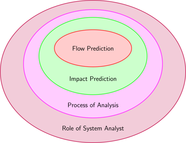
The methodological challenge of transportation systems is to conduct a systematic analysis in a particular situation which is valid, practical, and relevant and which assist in clarifying the issues to debated. The core of the system analysis is the prediction of flows, which must be complemented by the prediction for other impacts. Refer Fig. 1 Predication is only a part of the process of analysis and technical analysis is only a part of the broader problem, and the role of the professional transportation system analyst is to model the process of bringing about changes in the society through the means of transport.

1.5 Influence of TSA: Applications

Transportation system analysis can lead to different application specialties and they include:

1. highway engineering
2. freight transportation
3. marine transportation
4. transportation management
5. airport planning
6. port planning and development
7. transportation regulation
8. transportation economics
9. environmental impacts

1.6 Influence of TSA: Methodologies

Transportation system analysis can also lead to different methodological specialties and they include:

1. demand analysis, estimation and forecasting
2. transportation system performance like delays, waiting time, mobility, etc.
3. policy analysis and implementation
4. urban planning and development
5. land-use management

1.7 Influence of TSA: Methodologies

Finally, transportation system analysis can lead to different professional specialties and they include:

1. technical analyst
2. project managers
3. community interaction
4. policy analyst

2 The Scope of TSA

2.1 Background: A changing world

The strong interrelationship and the interaction between transportation and the rest of the society especially in a rapidly changing world is significant to a transportation planner. Among them four critical dimensions of change in transportation system can be identified; which form the background to develop a right perspective.

1. Change in the demand: When the population, income, and land-use pattern changes, the pattern of demand changes; both in the amount and spatial distribution of that demand.
2. Changes in the technology: As an example, earlier, only two alternatives (bus transit and rail transit) were considered for urban transportation. But, now new system like LRT, MRTS, etc offer a variety of alternatives.
3. Change in operational policy: Variety of policy options designed to improve the efficiency, such as incentive for car-pooling, road pricing etc.
4. Change in values of the public: Earlier all beneficiaries of a system was monolithically considered as users. Now, not one system can be beneficial to all, instead one must identify the target groups like rich, poor, young, work trip, leisure, etc.

2.2 Basic premise of a transportation system

The first step in formulation of a system analysis of transportation system is to examine the scope of analytical work. The basic premise is the explicit treatment of the total transportation system of region and the interrelations between the transportation and socio-economic context.

1. The total transportation system must be viewed as a single multi-modal system.
2. Considerations of transportation system cannot be separated from considerations of social, economic, and political system of the region.

This follows that the analysis of transportation system consists of the:

1. consideration all modes of transportation,
2. consideration all elements of transportation like persons, goods, carriers (vehicles), paths in the network facilities in which vehicles are going, the terminal, etc.,
3. consideration all movements of movements of passengers and goods for every O-D pair, and the
4. consideration the total trip for every flows for every O-D over all modes and facilitates.

As an example consider the the study of inter-city passenger transport in metro cities.

1. Consider all modes: i.e rail, road, air, buses, private automobiles, trucks, new modes like LRT, MRTS, etc.
2. Consider all elements like direct and indirect links, vehicles that can operate, terminals, transfer points, intra-city transit like taxis, autos, urban transit.
3. Consider diverse pattern of O-D of passenger and good.
4. Consider service provided for access, egress, transfer points and mid-block travel etc.

Once all these components are identified, the planner can focus on elements that are of real concern.

2.3 Interrelationship of T&A

Transportation system is tightly interrelated with socio-economic system. Transportation affect the growth and changes of socio-economic system, and will triggers changes in transportation system. The whole system of interest can be defined by these basic variables:

1. The transportation system including different modes, facilities like highways, etc.
2. The socio-economic activity system like work, land-use, housing, schools, etc. Activity system is defined as the totality of social, economic, political, and other transactions taking place over space and time in a given region.
3. The flow pattern which includes O-D, routes, volume or passenger/goods, etc.

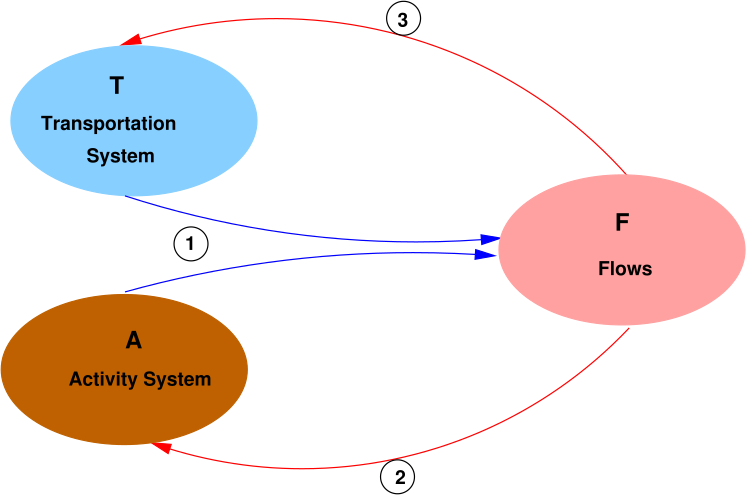
Three kinds or relationships can be identified as shown in Fig. 2 and can be summaries as follows:

1. \(F\) is determined by \(T\) and \(A\).
2. Current \(F\) will cause changes over time in \(A\) through the pattern of \(T\) and through the resources consumed in providing \(T\).
3. Current \(F\) will also cause changes over time in \(T\) due to changes in \(A\)

Note that \(A\) is not a simple variable as it looks. Also note that transportation is not the sole agency causing changes in \(A\).

2.4 Intervening TAF system

The mode of fulfilling the objective of intervening the system of TAF is important. The three major player in the TAF system are:

1. User: The users of the transportation system will decide when where and how to travel.
2. Operator: The operator of a particular facility or service operator will decide the mode of operation, routes, schedule, facilities, etc.
3. Government Government will decided on taxes, subsidies, construction of new facilities, governing law, fares, etc.

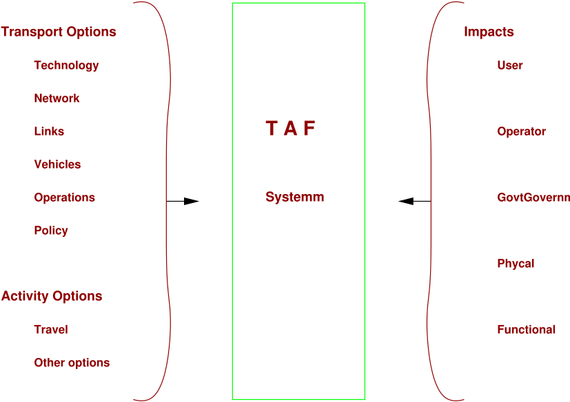
Their intervention can be in either transportation or activity system. The transportation options available to impart changes in the system are:

1. Technology (e.g. articulated bus, sky bus, etc.);
2. Network (e.g. grid or radial);
3. Link characteristics (e.g. signalized or flyover at an intersection);
4. Vehicles (e.g. increase the fleet size);
5. System operating policy (e.g. increase frequency or subsidy); and
6. Organizational policy (e.g. private or public transit system in a city).

On the other hand, some of the activity options are:

1. Travel demand: This is the aggregate result of all the individual travel decisions. The decision can be travel by train or bus, shortest distance route or shortest travel time route, when (time) and how (mode) to travel, etc.
2. Other options: Most of the social, economic, and political factors in the activity system decide when, how, or where to conduct activities. For example, the choice of school is affected by the transportation facility, or the price of real estate influenced by the transportation facilities.

The impacts of the transportation and activity options mentioned above diverse impact as illustrated in fig. 3

3 Prediction of flows

3.1 Concepts

Any proposed change in transportation system will trigger a change in the flows. Similarly, any change in the activity system also will cause changes in the flows. A sound procedure is needed to predict the flows resulting from changes in the transportation system or activity system or both. Thus, the core of the transportation systems analysis is the prediction of changes in flows due to changes proposed in the transportation system or the changes projected in the activity system. Consider the present transportation system \(T\) and an activity system \(A\). Let the proposed changes to the transportation system be \(\Delta {T}\) and new transportation system is defined as \(T'\). Similarly, let the projected changes in the activity system be \(\Delta {A}\) and the new activity system is defined as \(A'\). This implies that, there will be also changes in flow, denoted by \(F'\). This can be formally stated as:

The assumption here is that there exists an equilibrium between \(T\), \(A\), and \(F\). In other words, at any point in time, the specification of transportation system \(T\) and of activity system \(A\) implies the existence of a unique pattern of flows, \(F\). The basic hypothesis underlying this statement is that there is a market for transportation which can be separated out from other markets. This is type 1 relationship and it can be separated out from type 2 and type 3 relationships (Fig. 2).

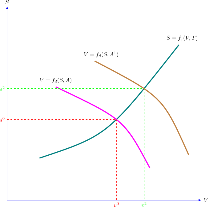
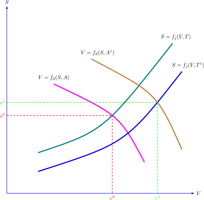
Introducing two more variables, the first indicates the service characteristics expressed by \(F\) like travel time, fare, comfort, etc. which is denoted as \(S\) and the volume of flow in the network denoted as \(V\), following relations can be stated.

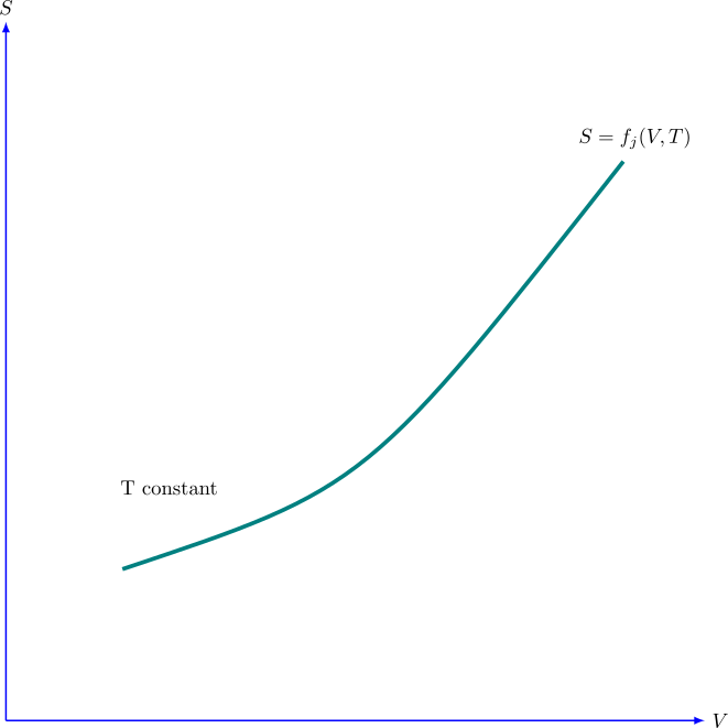
1. Specification of transportation system \(T\) establishes service function \(f_j\) which indicates how the level of service varies as a function of the transportation option and the volume of flows; i.e. \begin {equation} S=f_j(T,V) \end {equation}
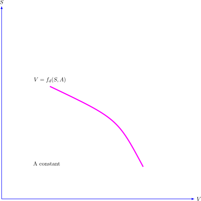
2. Specification of the activity system options, \(A\) establishes demand function, \(f_d\), which gives the volume of flow as function of activity system and level of service; i.e. \begin {equation} V=f_d(A,S) \end {equation}
3. The flow pattern \(F\) consists of the volume \(V\) using the system and level of service \(S\); i.e. \begin {equation} F=(V,S) \end {equation}

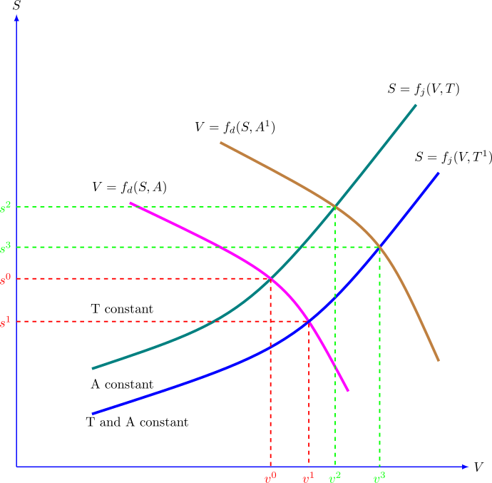
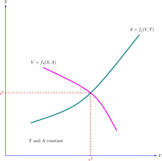
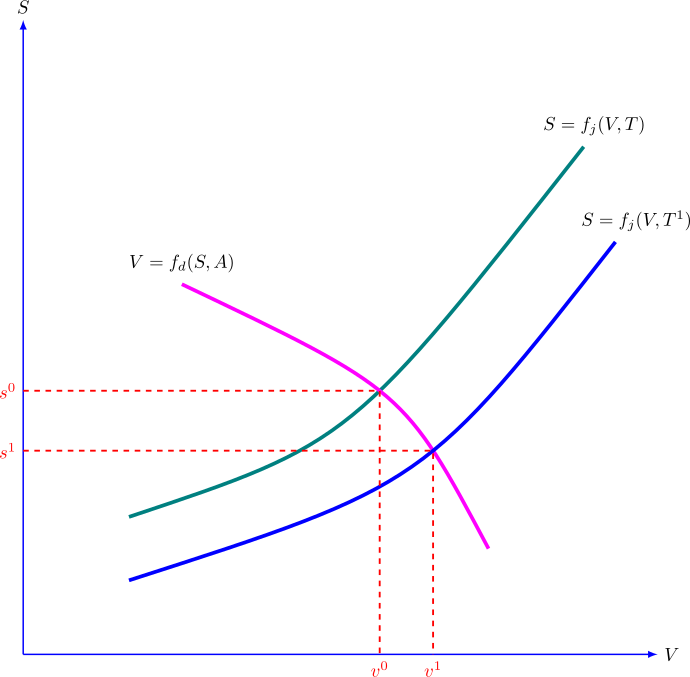
for a particular \(T\) and \(A\), the flow pattern that will actually occur can be found by the solution of service function and demand function:

The above relations are shown in Fig. ??.

3.2 Example

To illustrate the above concepts, we can consider a road connecting two cities. First, consider the transportation system. Assume that the level of service \(S\) is expressed by the travel time \(t\) between these two cities (this is the service level). The road has two lanes with one lane on each direction and has a length of 10 units (this is the transportation system). Assume one direction for our consideration. The general form of the service function can be: \begin {equation} f_j\implies t=m+n~v. \label {qeSupFun} \end {equation} Here, the parameter defining the transportation system are \(m\) and n. For the current example, assume \(m\) is 10 minutes and \(n\) is 0.01 minutes per vehicle per hour. Thus, the service function \(f_j\implies t=10+0.01~v\) which means that the travel time \(t\) in minutes will reduce with flow in vehicles per hour. Now consider the activity system. The cities are characterised by their populations, employment levels, etc. Here, we consider the demand in one direction from travel from city one to two. The general form the the demand function can be: \begin {equation} f_d\implies v=a+b~t. \label {qeDemFun} \end {equation} Here, the parameters reflecting the travel behaviours are \(a\) and b. For this example, assume \(a\) is 5000 vehicles per hour and \(b\) is -100 vehicles per hour per minutes. This means that the demand for travel will reduce from 5000 vehicle per hour by 100 vehicles for every unit increase in travel time. Thus, the demand function is give as \(f_d\implies v=5000-100~t\).

Now the resulting flow pattern F is define by the volume \(v\) of the trips from city one to two in vehicle per and the level of service they experience can be expressed by the travel time \(t\) in minutes. Thus, the flow depends on the volume using the facility and the travel time (\(F=(v,t)\)). At equilibrium, the flow pattern is represented by \((v^o,t^o)\) corresponding to the current transport and activity system options. Mathematically, this can be represented as two equations, namely, \(t^o=m+n~v^o=10+0.01~v^o\) and \(v^o=a+b~t^o=5000-100~t^o\), corresponding the demand and supply functions respectively. The equilibrium solution will have the value of \(t^o\) and \(v^o\) that satisfies both the equations. This can be solved algebraically or graphically (see figure ??). Numerically, the equilibrium solution is \(t^o=30\) minutes and \(v^o=2000\) vehicles per hour.

4 Summary

This chapter gives a broad framework on what is transportation systems modeling and the theoretical basis for that. The modeling involves defining a transport system, activity system and their interactions resulting in the flow. Note that this modeling frameworks is analogous to the demand supply concept in economics that determines the price of a commodity and the quantity produced.

4.1 Under construction

Exercises

1. Consider a highway connecting city 1 and city 2. The travel time \(t\) in minutes between these two cities is give as \(t=15+6v\) where \(v\) is the traffic volume and \(6v\) gives the additional time in sec/vehicle/hour. The traffic volume between these two cities is given by \(v=5000-100t\) where volume is in vehicle/hour and travel time is vehicle/hour/minute. Suppose the highway is widened and the resulting travel time function is \(t=3+v\), the units same as earlier, find the initial and final travel time and traffic volume.
2. The the service function of a road connecting two cities is give as \(f_j\implies t=m+n~v\), where \(t\) is the travel time between the cities and \(v\) is the volume of vehicles using that road. What are the physical significance of the parameters \(m\) and \(n\)
3. The demand function representing the travel between two cities is give as \(f_d\implies v=a+b~t\), where \(t\) is the travel time between the cities and \(v\) is the number of trips from city one to two. What are the physical significance of the parameters \(m\) and \(n\)
4. See page 148 Example 1 of the document Transportation Economics
5. See page 149 Example 2 of the document Transportation Economics
6. Select a current transportation issue for modeling and do the following. (i) Identify the transportation system components, (ii) Activity system that is interest to the transportaion issue, (iii) What could be a suitable service function, (iv) What could be a suitable demand function, (v) Visualize how the activity system may change, (vi) Propose some transport improvement options, (vii) Illustrate flow predictions.

References

1. Jotin C Khisty and Kent B Lall. Transportation Engineering An Introduction. Prentice Hall India, 2006.
2. M L Manheim. Fundamentals of transportation systems analysis Vol.1. MIT Press, 1978.

Web links

1. Transportation Economics
2. Economics Basics: Supply and Demand
3. Supply and demand

Acknowledgments

I wish to thank several of my students and staff of NPTEL for their contribution in this lecture. I also appreciate your constructive feedback which may be sent to tvm@civil.iitb.ac.in. Prof. Tom V. Mathew, Department of Civil engineering, Indian Instiute of Technology Bombay, India.