Introduction to Travel Demand Modeling

Lecture Notes in Transportation Systems Engineering

Prof. Tom V. Mathew

Contents

1 Overview
2 Transport modeling
3 Transport demand and supply
4 Travel demand modeling
5 Summary
Exercises
References
Acknowledgments
_________________________________________________________________________________________

1 Overview

This chapter provides an introduction to travel demand modeling, the most important aspect of transportation planning. First we will discuss about what is modeling, the concept of transport demand and supply, the concept of equilibrium, and the traditional four step demand modeling. We may also point to advance trends in demand modeling.

2 Transport modeling

Modeling is an important part of any large scale decision making process in any system. There are large number of factors that affect the performance of the system. It is not possible for the human brain to keep track of all the player in system and their interactions and interrelationships. Therefore we resort to models which are some simplified, at the same time complex enough to reproduce key relationships of the reality. Modeling could be either physical, symbolic, or mathematical In physical model one would make physical representation of the reality. For example, model air crafts used in wind tunnel is an example of physical models. In symbolic model, complex relations could be represented with the help of symbols. Drawing time-space diagram of vehicle movement is a good example of symbolic models. Mathematical models are the most common type of modeling where with the help of variables, parameters, and equations one could represent highly complex relations. Newton’s equations of motion or Einstein’s equation E = mc2, can be considered as examples of mathematical model. No model is a perfect representation of the reality. The important objective is that models seek to isolate key relationships, and not to replicate the entire structure. Transport modeling is the study of the behavior of individuals in making decisions regarding the provision and use of transport. Therefore, unlike other engineering models, transport modeling tools have evolved from many disciplines like economics, psychology, geography, sociology, and statistics.

3 Transport demand and supply

The concept of demand and supply are fundamental to economic theory and is widely applied in the field to transport economics. In the area of travel demand and the associated supply of transport infrastructure, the notions of demand and supply could be applied. However, we must be aware of the fact that the transport demand is a derived demand, and not a need in itself. That is, people travel not for the sake of travel, but to participate in activities at various locations

The concept of equilibrium is central to the supply-demand analysis. It is a normal practice to plot the supply and demand curve as a function of cost and the intersection is then plotted as the equilibrium point (Figure ??).

SVG-Viewer needed.

Figure 1: Demand Supply Equilibrium

The demand for travel (T) is a function of cost (C) is easy to conceive. Classical approach defines the supply function as giving the quantity (T) which would be produced, given a market price (C). Since transport demand is a derived demand, and the benefit of transportation on the non-monetary terms (time in particular), the supply function takes the form in which (T) is the unit cost associated with meeting a demand (C). Thus, the supply function encapsulates response of the transport system to a given level of demand. In other words, supply function will answer the question what will be the level of service of the system, if the estimated demand is loaded to the system. The most common supply function is the link travel time function which relates the link volume (v) and travel time (t = f(v)).

4 Travel demand modeling

Travel demand modeling aims to establish the spatial distribution of travel explicitly by means of an appropriate system of zones. Modeling of demand thus implies a procedure for predicting what travel decisions people would like to make given the generalized travel cost of each alternatives. The base decisions include the choice of destination, the choice of the mode, and the choice of the route. Although various modeling approaches are adopted, we will discuss only the classical transport model popularly known as four-stage model (FSM).

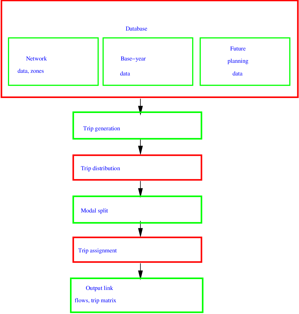
The general form of the four stage model is given in Figure 2.

PIC

Figure 2: General form of the four stage modeling

The classic model is presented as a sequence of four sub models: trip generation, trip distribution, modal split, trip assignment. The models starts with defining the study area and dividing them into a number of zones and considering all the transport network in the system. The database also include the current (base year) levels of population, economic activity like employment, shopping space, educational, and leisure facilities of each zone. Then the trip generation model is evolved which uses the above data to estimate the total number of trips generated and attracted by each zone. The next step is the allocation of these trips from each zone to various other destination zones in the study area using trip distribution models. The output of the above model is an origin-destination trip matrix (O-D Matrix) which denote the trips from each zone to every other zones. In the succeeding step the trips are allocated to different modes based on the modal attributes using the modal split models. This is essentially slicing the trip matrix for various modes generated to a mode specific trip matrix. Finally, each trip matrix is assigned to the route network of that particular mode using the trip assignment models. The step will give the loading on each link of the network.

The classical model would also be viewed as answering a series of questions (decisions) namely how many trips are generated, where they are going, on what mode they are going, and finally which route they are adopting. The current approach is to model these decisions using discrete choice theory, which allows the lower level choices to be made conditional on higher choices. For example, route choice is conditional on the mode choice. This hierarchical choices of trip is shown in Figure ??.

SVG-Viewer needed.

Figure 3: Hierarchical choices of trip making

The highest level is to find all the trips Ti originating from a zone and is estimated based on the data and aggregate cost term Ci***. Based on the aggregate travel cost Cij** from zone i to the destination zone j, the probability pji of trips going to zone j is computed and subsequently the trips Tij** from zone i to zone j by all modes and all routes are computed. Next, the mode choice model compute the probability pmij of choosing mode m based on the travel cost Cijm* from zone i to zone j, by mode m is determined. Similarly, the route choice gives the trips Tijmr from zone i to zone j by mode m through route r. In this final stage, the travel demand is loaded to the supply model, and as stated earlier, will produce the volume using the facility which can be used to compute appropriate performance levels. The performance of the network is usually measured in travel time which could be converted to travel cost. Although not a popular practice, one could feed this back into the higher levels to achieve real equilibrium of the supply and demand.

5 Summary

In a nutshell, travel demand modeling aims at explaining where the trips come from, where they go, what mode they choose, and which routes the choose. It provides a zone wise analysis of the trips followed by distribution of the trips, split the trips mode wise based on the choice of the travelers and finally assigns the trips to the network. This process helps to understand the effects of future developments in the transport networks on the trips as well as the influence of the choices of the public on the flows in the network.

Exercises

  1. Multiple choice or fill-in-the blanks kind of questions:
    1. Link travel time function relates travel time and …( a. link volume, b. link cost, c. level of service, d. none of the above.)
    2. What is the first stage of four-stage travel demand modeling? ( a. Trip generation, b. Trip distribution, c. Modal split, d. Traffic assignment.)
  2. Draw a neat sketch of Mumbai city and illustrate the concept of internal zones, external zones, cordon line, and screen lines.
  3. Illustrate the concept of four-stage travel demand modelling for flow predication with help of a flow chart. Show also the input and output of the model. Mark also with the help of suitable mathematical notation what each stage is accomplishing.

References

  1. David A Hensher and Kenneth J Button. Handbook of Transport Modelling, volume 1. Elsevier, London, 2 edition, 2007.
  2. J D Ortuzar and L G Willumnsen. Modeling Transport. John Wiley and Sons, New York, 1994.

Web links

  1. A presentation on Travel Demand Modeling by Prof. Moshe Ben-Akiva of MIT.
  2. Youtube Video lecture on Overview of the four-step transport demand model by Dr. Ian Espanda of Australian Road Research Board.

Acknowledgments

I wish to thank several of my students and staff of NPTEL for their contribution in this lecture. I also appreciate your constructive feedback which may be sent to tvm@civil.iitb.ac.in

Prof. Tom V. Mathew
Department of Civil Engineering
Indian Institute of Technology Bombay, India

____________________________________________________________________________________________

Fri Mar 8 12:42:52 IST 2019