
The third stage in travel demand modeling is modal split. The trip matrix or O-D matrix obtained from the trip distribution is sliced into number of matrices representing each mode. First the significance and factors affecting mode choice problem will be discussed. Then a brief discussion on the classification of mode choice will be made. Two types of mode choice models will be discussed in detail. ie binary mode choice and multinomial mode choice. The chapter ends with some discussion on future topics in mode choice problem.
The choice of transport mode is probably one of the most important classic models in transport planning. This is because of the key role played by public transport in policy making. Public transport modes make use of road space more efficiently than private transport. Also they have more social benefits like if more people begin to use public transport , there will be less congestion on the roads and the accidents will be less. Again in public transport, we can travel with low cost. In addition, the fuel is used more efficiently. Main characteristics of public transport is that they will have some particular schedule, frequency etc.
On the other hand, private transport is highly flexible. It provides more comfortable and convenient travel. It has better accessibility also. The issue of mode choice, therefore, is probably the single most important element in transport planning and policy making. It affects the general efficiency with which we can travel in urban areas. It is important then to develop and use models which are sensitive to those travel attributes that influence individual choices of mode.
The factors may be listed under three groups:
Qualitative factors which are less easy to measure are:
A good mode choice should include the most important of these factors.
Traditionally, the objective of transportation planning was to forecast the growth in demand for car trips so that investment could be planned to meet the demand. When personal characteristics were thought to be the most important determinants of mode choice, attempts were made to apply modal-split models immediately after trip generation. Such a model is called trip-end modal split model. In this way different characteristics of the person could be preserved and used to estimate modal split. The modal split models of this time related the choice of mode only to features like income, residential density and car ownership.
The advantage is that these models could be very accurate in the short run, if public transport is available and there is little congestion. Limitation is that they are insensitive to policy decisions example: Improving public transport, restricting parking etc. would have no effect on modal split according to these trip-end models.
This is the post-distribution model; that is modal split is applied after the distribution stage. This has the advantage that it is possible to include the characteristics of the journey and that of the alternative modes available to undertake them. It is also possible to include policy decisions. This is beneficial for long term modeling.
Mode choice could be aggregate if they are based on zonal and inter-zonal information. They can be called disaggregate if they are based on household or individual data.
Binary logit model is the simplest form of mode choice, where the travel choice between two modes is made. The traveler will associate some value for the utility of each mode. if the utility of one mode is higher than the other, then that mode is chosen. But in transportation, we have disutility also. The disutility here is the travel cost. This can be represented as
|
| (1) |
where tijv is the in-vehicle travel time between i and j, t ijw is the walking time to and from stops, t ijt is the waiting time at stops, Fij is the fare charged to travel between i and j, ϕj is the parking cost, and δ is a parameter representing comfort and convenience. If the travel cost is low, then that mode has more probability of being chosen. Let there be two modes (m=1,2) then the proportion of trips by mode 1 from zone i to zone j is(Pij1) Let c ij1 be the cost of traveling from zone i to zonej using the mode 1, and cij2 be the cost of traveling from zonei to zone j by mode 2,there are three cases:
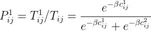
This relationship is normally expressed by a logit curve as shown in figure 1 Therefore the proportion of trips by mode 1 is given by
 | (2) |
This functional form is called logit, where cij is called the generalized cost and β is the parameter for calibration. The graph in figure 1 shows the proportion of trips by mode 1 (Tij1∕T ij) against cost difference.
Let the number of trips from zone
| | | | | |
|
| car | 20 | - | 18 | 4 | |
| bus | 30 | 5 | 3 | 9 | |
| | 0.03 | 0.04 | 0.06 | 0.1 | 0.1 |
| | | | | | | | |
|
| ar | 20 | - | 18 | 4 | 2.08 | .52 | 2600 | |
| bus | 30 | 5 | 3 | 9 | 2.18 | .475 | 2400 | |
| | .03 | .04 | .06 | .1 | .1 | |||
 = 0.52
 = 0.475
When the fare of bus gets reduced to 6,
 = 0.55
The results are tabulated in table
The binary model can easily be extended to multiple modes. The equation for such a model can be written as:
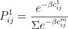 | (3) |
Let the number of trips from
| | | | | |
|
| coefficient | 0.03 | 0.04 | 0.06 | 0.1 | 0.1 |
| car | 20 | - | - | 18 | 4 |
| bus | 30 | 5 | 3 | 6 | - |
| train | 12 | 10 | 2 | 4 | - |
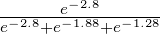 = 0.1237
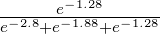
 = 0.3105
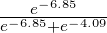
 = 0.5657
| | | | | | | | | |
|
| coeff | 0.03 | 0.04 | 0.06 | 0.1 | 0.1 | - | - | - | - |
| car | 20 | - | - | 18 | 4 | 2.8 | 0.06 | 0.1237 | 618.5 |
| bus | 30 | 5 | 3 | 6 | - | 1.88 | 0.15 | 0.3105 | 1552.5 |
| train | 12 | 10 | 2 | 4 | - | 1.28 | 0.28 | 0.5657 | 2828.5 |
Modal split is the third stage of travel demand modeling. The choice of mode is influenced by various factors. Different types of modal split models are there. Binary logit model and multinomial logit model are dealt in detail in this chapter.
| | | | | |
|
| coefficient | 0.05 | 0.04 | 0.07 | 0.2 | 0.2 |
| car | 25 | - | - | 22 | 6 |
| bus | 35 | 8 | 6 | 8 | - |
| train | 17 | 14 | 5 | 6 | - |
 = 0.059
 = 0.9403
 = 0.02003
 = 0.979
Case 1:
Case 2:
Hence
I wish to thank several of my students and staff of NPTEL for their contribution in this lecture. I
also appreciate your constructive feedback which may be sent to
Prof. Tom V. Mathew
Department of Civil Engineering
Indian Institute of Technology Bombay, India
____________________________________________________________________________________________
Fri Mar 8 12:14:00 IST 2019