This chapter covers a numerical method to solve traffic assignmenr by user equilibrium or system
optimum method. The method is known as Frank-Wolfe algorithm or convex combination
algorithm.
2 All-OR-Nothing Assignment
Numerical illustartion: under preparation.
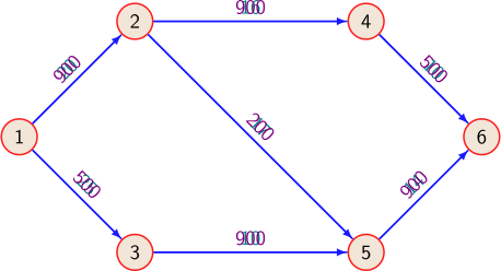
Figure 1: Network Flow Conservation Problem
3 Frank-Wolfe Algorithm for UE
Step 0: Initilize
Set \(n=1\), \(t_a=t_a(0)~~~\forall a\)
Do \(AON \rightarrow \{x_a^n\}\)
Step 1: Update
Set \(t_a^n=t_a(x_a^n)\)
Step 2: Direction finding
Do \(AON\) based on \(t_a^n \rightarrow \{y_a^n\}\)
If \(| x_a^{n+1}-x_a^n |\le \epsilon ~~~\forall a\) then STOP
else set \(n=n+1\), go to step 1.
3.1 Numerical Example
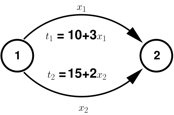
To demonstrate the Frank-Wolfe algorithm, consider an example network give in figure 2. This network
has two nodes having two paths as links. The travel time is a function of link flow for both the links and is
given as: \(t_1=10+3x_1\) and \(t_2=15+2x_2\), and total flows from 1 to 2 is given as \(q_{12}=12\). Do an UE assignment using Frank-Wolfe algorithm
and show two full iterations.
Figure 2: Two link problem for solving UE assignment by Franl-Wolfe algorithm
Solution
Step 0: Initilize
Set \(n=1\), \(t_1^1=t_1^1(0)=10\), \(t_2^1=t_2^1(0)=15\)
Solving by taking \(\frac {dz}{d\alpha }=0\) \(\implies \alpha ^*=0.517\)
Step 4: Move
Get \(x_1=12-12\alpha =12-12\times 0.517=5.796\)
Get \(x_2=12\alpha =12\times 0.517=6.204\)
Step 5: Convergence
If \(| x_a^{n+1}-x_a^n |\le \epsilon ~~~\forall a\) then STOP
else set \(n=n+1\), go to step 1.
Exercises
Not Available
References
Yosef Sheffi. Urban transportation networks: Equilibrium analysis with mathematical
programming methods. New Jersey, 1984.
R Thomas. Traffic Assignment Techniques. Avebury Technical publication,England, 1991.
Acknowledgments
I wish to thank several of my students and staff of NPTEL for their contribution in this lecture. I
also appreciate your constructive feedback which may be sent to tvm@civil.iitb.ac.in. Prof.
Tom V. Mathew, Department of Civil engineering, Indian Instiute of Technology Bombay,
India.