The safe and efficient operation of vehicles on the road depends very much on the visibility of the road ahead of the driver. Thus the geometric design of the road should be done such that any obstruction on the road length could be visible to the driver from some distance ahead . This distance is said to be the sight distance.
Sight distance available from a point is the actual distance along the road surface, over which a driver from a specified height above the carriage way has visibility of stationary or moving objects. Three sight distance situations are considered for design:
The most important consideration in all these is that at all times the driver traveling at the design speed of the highway must have sufficient carriageway distance within his line of vision to allow him to stop his vehicle before colliding with a slowly moving or stationary object appearing suddenly in his own traffic lane.
The computation of sight distance depends on:
Reaction time of a driver is the time taken from the instant the object is visible to the driver to the instant when the brakes are applied. The total reaction time may be split up into four components based on PIEV theory. In practice, all these times are usually combined into a total perception-reaction time suitable for design purposes as well as for easy measurement. Many of the studies shows that drivers require about 1.5 to 2 secs under normal conditions. However, taking into consideration the variability of driver characteristics, a higher value is normally used in design. For example, IRC suggests a reaction time of 2.5 secs.
The speed of the vehicle very much affects the sight distance. Higher the speed, more time will be required to stop the vehicle. Hence it is evident that, as the speed increases, sight distance also increases.
The efficiency of the brakes depends upon the age of the vehicle, vehicle characteristics etc. If the brake efficiency is 100%, the vehicle will stop the moment the brakes are applied. But practically, it is not possible to achieve 100% brake efficiency. Therefore the sight distance required will be more when the efficiency of brakes are less. Also for safe geometric design, we assume that the vehicles have only 50% brake efficiency.
The frictional resistance between the tyre and road plays an important role to bring the vehicle to stop. When the frictional resistance is more, the vehicles stop immediately. Thus sight required will be less. No separate provision for brake efficiency is provided while computing the sight distance. This is taken into account along with the factor of longitudinal friction. IRC has specified the value of longitudinal friction in between 0.35 to 0.4.
Gradient of the road also affects the sight distance. While climbing up a gradient, the vehicle can stop immediately. Therefore sight distance required is less. While descending a gradient, gravity also comes into action and more time will be required to stop the vehicle. Sight distance required will be more in this case.
Stopping sight distance (SSD) is the minimum sight distance available on a highway at any spot having sufficient length to enable the driver to stop a vehicle traveling at design speed, safely without collision with any other obstruction.
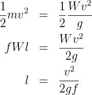
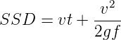
There is a term called safe stopping distance and is one of the important measures in traffic engineering. It is the distance a vehicle travels from the point at which a situation is first perceived to the time the deceleration is complete. Drivers must have adequate time if they are to suddenly respond to a situation. Thus in highway design, sight distance atleast equal to the safe stopping distance should be provided. The stopping sight distance is the sum of lag distance and the braking distance. Lag distance is the distance the vehicle traveled during the reaction time t and is given by vt, where v is the velocity in m∕sec2. Braking distance is the distance traveled by the vehicle during braking operation. For a level road this is obtained by equating the work done in stopping the vehicle and the kinetic energy of the vehicle. If F is the maximum frictional force developed and the braking distance is l, then work done against friction in stopping the vehicle is Fl = fWl where W is the total weight of the vehicle. The kinetic energy at the design speed is
 | (1) |
where v is the design speed in m∕sec2, t is the reaction time in sec, g is the acceleration due to gravity and f is the coefficient of friction. The coefficient of friction f is given below for various design speed.
| Speed, kmph | <30 | 40 | 50 | 60 | >80 |
| f | 0.40 | 0.38 | 0.37 | 0.36 | 0.35 |
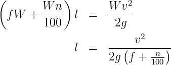
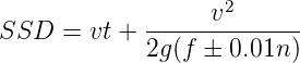
When there is an ascending gradient of say +n%, the component of gravity adds to braking action and hence braking distance is decreased. The component of gravity acting parallel to the surface which adds to the the braking force is equal to W sin α ≈ W tan α = Wn∕100. Equating kinetic energy and work done:
 | (2) |
The overtaking sight distance is the minimum distance open to the vision of the driver of a vehicle intending to overtake the slow vehicle ahead safely against the traffic in the opposite direction. The overtaking sight distance or passing sight distance is measured along the center line of the road over which a driver with his eye level 1.2 m above the road surface can see the top of an object 1.2 m above the road surface.
The factors that affect the OSD are:
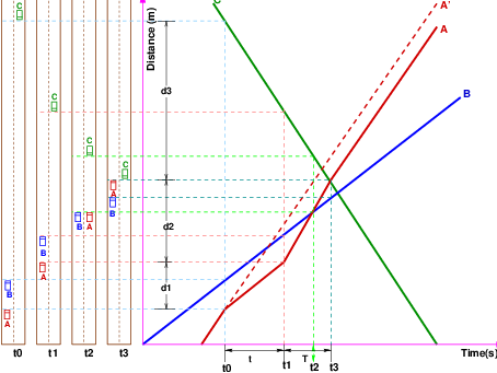
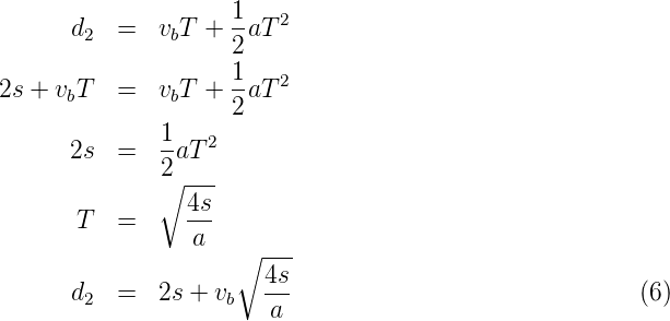
The dynamics of the overtaking operation is given in the figure which is a time-space diagram. The x-axis denotes the time and y-axis shows the distance traveled by the vehicles. The trajectory of the slow moving vehicle (B) is shown as a straight line which indicates that it is traveling at a constant speed. A fast moving vehicle (A) is traveling behind the vehicle B. The trajectory of the vehicle is shown initially with a steeper slope. The dotted line indicates the path of the vehicle A if B was absent. The vehicle A slows down to follow the vehicle B as shown in the figure with same slope from t0 to t1. Then it overtakes the vehicle B and occupies the left lane at time t3. The time duration T = t3 - t1 is the actual duration of the overtaking operation. The snapshots of the road at time t0,t1, and t3 are shown on the left side of the figure. From the Figure 1, the overtaking sight distance consists of three parts.
Therefore:


 | (8) |
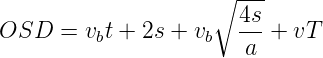
where vb is the velocity of the slow moving vehicle in m∕sec2, t the reaction time of the driver in sec, s is the spacing between the two vehicle in m given by equation 5 and a is the overtaking vehicles acceleration in m∕sec2. In case the speed of the overtaken vehicle is not given, it can be assumed that it moves 16 kmph slower the the design speed.
The acceleration values of the fast vehicle depends on its speed and given in Table 2.
| Speed | Maximum overtaking |
| (kmph) | acceleration (m/sec2) |
| 25 | 1.41 |
| 30 | 1.30 |
| 40 | 1.24 |
| 50 | 1.11 |
| 65 | 0.92 |
| 80 | 0.72 |
| 100 | 0.53 |
Note that:
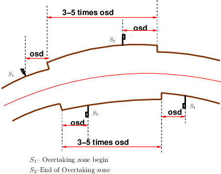
Overtaking zones are provided when OSD cannot be provided throughout the length of the highway. These are zones dedicated for overtaking operation, marked with wide roads. The desirable length of overtaking zones is 5 time OSD and the minimum is three times OSD (Figure 2).
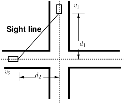
At intersections where two or more roads meet, visibility should be provided for the drivers approaching the intersection from either sides. They should be able to perceive a hazard and stop the vehicle if required. Stopping sight distance for each road can be computed from the design speed. The sight distance should be provided such that the drivers on either side should be able to see each other. This is illustrated in the figure 3.
Design of sight distance at intersections may be used on three possible conditions:
One of the key factors for the safe and efficient operation of vehicles on the road is sight distance. Sight distances ensure overtaking and stopping operations at the right time. Different types of sight distances and the equations to find each of these had been discussed here.


I wish to thank several of my students and staff of NPTEL for their contribution in this lecture. I also appreciate your constructive feedback which may be sent to tvm@civil.iitb.ac.in
Prof. Tom V. Mathew
Department of Civil Engineering
Indian Institute of Technology Bombay, India
____________________________________________________________________________________________
Thu Jan 10 12:41:42 IST 2019