Contents

1 Overview

The objective of dry mix design is to determine the amount of various sizes of mineral aggregates to use to get a mix of maximum density. The dry mix design involves three important steps, viz. selection of aggregates, aggregates gradation, and proportion of aggregates, which are discussed below.

2 Selection of aggregates

The desirable qualities of a bituminous paving mixture are dependent to a considerable degree on the nature of the aggregates used. Aggregates are classified as coarse, fine, and filler. The function of the coarse aggregates in contributing to the stability of a bituminous paving mixture is largely due to interlocking and frictional resistance of adjacent particles. Similarly, fines or sand contributes to stability failure function in filling the voids between coarse aggregates. Mineral filler is largely visualized as a void filling agent. Crushed aggregates and sharp sands produce higher stability of the mix when compared with gravel and rounded sands.

3 Aggregate gradation

The properties of the bituminous mix including the density and stability are very much dependent on the aggregates and their grain size distribution. Gradation has a profound effect on mix performance. It might be reasonable to believe that the best gradation is one that produces maximum density. This would involve a particle arrangement where smaller particles are packed between larger particles, thus reducing the void space between particles. This create more particle-to-particle contact, which in bituminous pavements would increase stability and reduce water infiltration. However, some minimum amount of void space is necessary to:

• provide adequate volume for the binder to occupy,
• promote rapid drainage, and
• provide resistance to frost action for base and sub base courses.

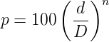
A dense mixture may be obtained when this particle size distribution follows Fuller law which is expressed as:

(1)

where, p is the percent by weight of the total mixture passing any given sieve sized, D is the size of the largest particle in that mixture, and n is the parameter depending on the shape of the aggregate (0.5 for perfectly rounded particles). Based on this law Fuller-Thompson gradation charts were developed by adjusting the parameter n for fineness or coarseness of aggregates. Practical considerations like construction, layer thickness, workability, etc, are also considered. For example Table  1 provides a typical gradation for bituminous concrete for a thickness of 40 mm.

4 Proportioning of aggregates

After selecting the aggregates and their gradation, proportioning of aggregates has to be done and following are the common methods of proportioning of aggregates:

• Trial and error procedure: Vary the proportion of materials until the required aggregate gradation is achieved.
• Graphical Methods: Two graphical methods in common use for proportioning of aggregates are, Triangular chart method and Roch’s method. The former is used when only three materials are to be mixed.
• Analytical Method: In this method a system of equations are developed based on the gradation of each aggregates, required gradation, and solved by numerical methods. With the advent of computer, this method is becoming popular and is discussed below. The resulting solution gives the proportion of each type of material required for the given aggregate gradation.

5 Example 1

The gradation required for a typical mix is given in Table  2 in column 1 and 2. The gradation of available for three types of aggregate A, B, and C are given in column 3, 4, and 5. Determine the proportions of A,B and C if mixed will get the required gradation in column 2.

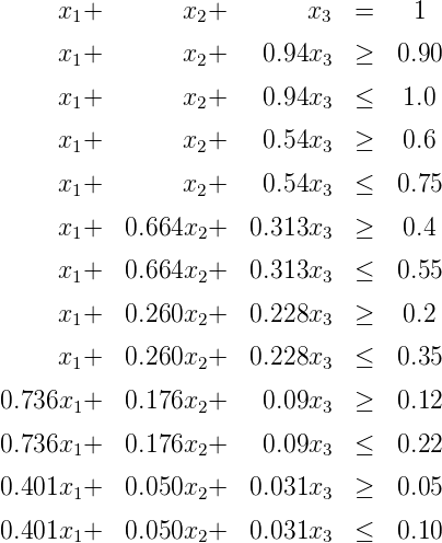
Solution The solution is obtained by constructing a set of equations considering the lower and upper limits of the required gradation as well as the percentage passing of each type of aggregate. The decision need to take is the proportion of aggregate A, B, C need to be blended to get the gradation of column 2. Let x₁, x₂, x₃ represent the proportion of A, B, and C respectively. Equation of the form ax₁ + bx₂ + cx₃ ≤ p_l or ≥ p_v can be written for each sieve size, where a, b, c is the proportion of aggregates A, B, and C passing for that sieve size and p_l and p_v are the required gradation for that sieve size. This will lead to the following system of equations:

(2)

Solving the above system of equations manually is extremely difficult. Good computer programs are required to solve this. Software like solver in Excel and Matlab can be used. Soving this set of equations is outside the scope of this book. Suppose the solution to this problem is x₁ = 0.05, x₂ = 0.3, x₃ = 0.65. Then Table 3 shows how when these proportions of aggregates A, B, and C are combined, produces the required gradation.

6 Summary

Various steps involved in the dry mix design were discussed. Gradation aims at reducing the void space, thus improving the performance of the mix. Proportioning is done by trial and error and graphical methods.

7 Problems

1. Fullers law is expressed as
   1. p=100×ⁿ
   2. p=100×ⁿ
   3. p=100×ⁿ
   4. p=100×ⁿ

Solutions

1. Fullers law is expressed as
   1. p=100×ⁿ√
   2. p=100×ⁿ
   3. p=100×ⁿ
   4. p=100×ⁿ

-

Exercises

1. Not Available

References

1. Y. H Huang. Pavement analysis and Design. Prentice-Hall, Englewood Cliffs, New Jersey, 1993.

Acknowledgments

I wish to thank several of my students and staff of NPTEL for their contribution in this lecture. I also appreciate your constructive feedback which may be sent to tvm@civil.iitb.ac.in

Prof. Tom V. Mathew
Department of Civil Engineering
Indian Institute of Technology Bombay, India