The relationship between these parameters can be represented by the Speed is one of the basic parameters of traffic flow and time mean speed and space mean speed are the two representations of speed. Time mean speed and space mean speed and the relationship between them will be discussed in detail in this chapter. The relationship between the fundamental parameters of traffic flow will also be derived. In addition, this relationship can be represented in graphical form resulting in the fundamental diagrams of traffic flow.
As noted earlier, time mean speed is the average of all vehicles passing a point over a duration of time. It is the simple average of spot speed. Time mean speed \(v_t\) is given by, \begin {equation} v_t = \frac {1}{n}\sum _{i=1}^{n}{v_i}, \label {qetimemeanspeed} \end {equation} where \(v_i\) is the spot speed of \(i^{th}\) vehicle, and \(n\) is the number of observations. In many speed studies, speeds are represented in the form of frequency table. Then the time mean speed is given by, \begin {equation} v_t = \frac {\sum _{i=1}^{n}{q_i v_i}}{\sum _{i=1}^{n}{q_i}}, \end {equation} where \(q_i\) is the number of vehicles having speed \(v_i\), and \(n\) is the number of such speed categories.
The space mean speed also averages the spot speed, but spatial weightage is given instead of temporal. This is derived as below. Consider unit length of a road, and let \(v_i\) is the spot speed of \(i^{th}\) vehicle. Let \(t_i\) is the time the vehicle takes to complete unit distance and is given by \(\frac {1}{v_i}\). If there are \(n\) such vehicles, then the average travel time \(t_s\) is given by, \begin {equation} t_s=\frac {\Sigma {t_i}}{n}=\frac {\Sigma {\frac {1}{v_i}}}{n}. \end {equation} If \(t_{av}\) is the average travel time, then average speed \(v_s = \frac {1}{t_s}\). Therefore, from the above equation, \begin {equation} v_s = \frac {n}{\sum _{i=1}^{n}\frac {1}{v_i}}. \end {equation} This is simply the harmonic mean of the spot speed. If the spot speeds are expressed as a frequency table, then, \begin {equation} v_s = \frac {\sum _{i=1}^{n}{q_i}}{\sum _{i=1}^{n}{\frac {q_i}{v_i}}}, \end {equation} where \(q_i\) vehicle will have \(v_i\) speed and \(n_i\) is the number of such observations.
If the spot speeds are 50, 40, 60, 54 and 45, then find the time mean speed and space mean speed.
Solution Time mean speed \(v_t\) is the average of spot speed. Therefore, \(v_t = \frac {\Sigma {v_i}}{n} = \frac {50+40+60+54+45}{5} = \frac {249}{5}\) = 49.8. Space mean speed is the harmonic mean of spot speed. Therefore, \(v_s = \frac {n}{\Sigma {\frac {1}{v_i}}} = \frac {5}{{\frac {1}{50}}+{\frac {1}{40}}+{\frac {1}{60}}+{\frac {1}{54}}+{\frac {1}{45}}} = \frac {5}{0.12} = 48.82.\)
The results of a speed study is given in the form of a frequency distribution table. Find the time mean speed and space mean speed.
| speed range | frequency |
| 2-5 | 1 |
| 6-9 | 4 |
| 10-13 | 0 |
| 14-17 | 7 |
| Sl. | speed | average | flow | \(q_i~v_i\) | \(\frac {q_i}{v_i}\) |
| No. | range | speed (\(v_i\)) | (\(q_i\)) | ||
| 1 | 2-5 | 3.5 | 1 | 3.5 | 2.29 |
| 2 | 6-9 | 7.5 | 4 | 30.0 | 0.54 |
| 3 | 10-13 | 11.5 | 0 | 0 | 0 |
| 4 | 14-17 | 15.5 | 7 | 108.5 | 0.45 |
| total | 12 | 142 | 3.28 | ||
The time mean speed and space mean speed can be found out from the frequency table given below. First, the average speed is computed, which is the mean of the speed range. For example, for the first speed range, average speed, \(v_i = \frac {2+5}{2}\) = 3.5 seconds. The volume of flow \(q_i\) for that speed range is same as the frequency. The terms \(v_i.q_i\) and \(\frac {q_i}{v_i}\) are also tabulated, and their summations given in the last row. Time mean speed can be computed as, \(v_t = \frac {\Sigma {q_iv_i}}{\Sigma q_i} = \frac {142}{12} = 11.83. \) Similarly, space mean speed can be computed as, \(v_s = \frac {\Sigma {q_i}}{\Sigma {\frac {q_i}{v_i}}} = \frac {12}{3.28} = 3.65.\)
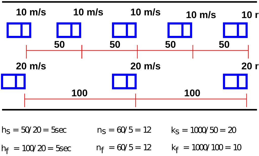
In order to understand the concept of time mean speed and space mean speed, following illustration will help. Let there be a road stretch having two sets of vehicle as in figure 1.
The first vehicle is traveling at 10m/s with 50 m spacing, and the second set at 20m/s with 100 m spacing. Therefore, the headway of the slow vehicle \(h_s\) will be 50 m divided by 10 m/s which is 5 sec. Therefore, the number of slow moving vehicles observed at A in one hour \(n_s\) will be 60/5 = 12 vehicles. The density \(K\) is the number of vehicles in 1 km, and is the inverse of spacing. Therefore, \(K_s = 1000/50\) = 20 vehicles/km. Therefore, by definition, time mean speed \(v_t\) is given by \(v_t = \frac {12\times 10+12\times 20}{24}~=~15~m/s\). Similarly, by definition, space mean speed is the mean of vehicle speeds over time. Therefore, \(v_s = \frac {20\times 10 + 10\times 20}{30}~=~13.3~m/s.\) This is same as the harmonic mean of spot speeds obtained at location A; ie \(v_s = \frac {24}{12\times \frac {1}{10}+12\times \frac {1}{20}} = 13.3~m/s.\) It may be noted that since harmonic mean is always lower than the arithmetic mean, and also as observed, space mean speed is always lower than the time mean speed. In other words, space mean speed weights slower vehicles more heavily as they occupy the road stretch for longer duration of time. For this reason, in many fundamental traffic equations, space mean speed is preferred over time mean speed.
The relation between time mean speed (\(v_t\)) and space mean speed (\(v_s\)) is given by the following relation:
where, \(\sigma _s\) is the standard deviation of the spot speed. The derivation of the formula is given in the next subsection. The standard deviation (\(\sigma ^2\)) can be computed in the following equation:
where, \(q_i\) is the frequency of the vehicle having \(v_i\) speed.
The relation between time mean speed and space mean speed can be derived as below. Consider a stream of vehicles with a set of sub-stream flow \(q_1\), \(q_2\), …\(q_i\), …\(q_n\) having speed \(v_1\),\(v_2\), …\(v_i\), …\(v_n\). The fundamental relation between flow(\(q\)), density(\(k\)) and mean speed \(v_s\) is, \begin {equation*} q=k\times v_s \end {equation*} Therefore for any sub-stream \(q_i\), the following relationship will be valid. \begin {equation*} q_i = k_i\times v_i \label {qetime} \end {equation*} The summation of all sub-stream flows will give the total flow \(q\): \begin {equation*} \Sigma q_i = q. \end {equation*} Similarly the summation of all sub-stream density will give the total density \(k\). \begin {equation*} \Sigma k_i = k. \end {equation*} Let \(f_i\) denote the proportion of sub-stream density \(k_i\) to the total density \(k\), \begin {equation*} f_i=\frac {k_i}{k}. \end {equation*} Space mean speed averages the speed over space. Therefore, if \(k_i\) vehicles has \(v_i\) speed, then space mean speed is given by, \begin {equation*} v_s=\frac {\Sigma k_i v_i}{k}. \end {equation*} Time mean speed averages the speed over time. Therefore, \begin {equation*} v_t=\frac {\Sigma q_i v_i}{q}. \end {equation*} Substituting \(q_i=k_i~v_i\), \(v_t\) can be written as, \begin {equation*} v_t = \frac {\Sigma {k_i}{{v_i}^2}}{q} \end {equation*} Rewriting the above equation and substituting \(f_i=\frac {k_i}{k}\), and then substituting \(q=k~v_s\), we get,
By adding and subtracting \(v_s\) and doing algebraic manipulations, \(v_t\) can be written as,
Note that, in the first term of the above equation, \(\Sigma f_i=1\) by definition. The numerator of the second term is the square of the standard deviation of \(v_i\) with respect to \(v_s\). The third term of the above equation is zero because \(\Sigma f_i(v_i-v_s)\) is zero by definition, since \(v_s\) is the mean of \(v_i\). Therefore, \begin {equation} v_t=v_s + \frac {\sigma _s^2}{v_s} \end {equation} Hence, time mean speed is space mean speed plus standard deviation of the spot speed divided by the space mean speed. Time mean speed will be always greater than space mean speed since standard deviation cannot be negative. If all the speed of the vehicles are the same, then spot speed, time mean speed and space mean speed will also be same.
For the data given below,compute the time mean speed and space mean speed. Also verify the relationship between them. Finally compute the density of the stream.
| speed range (\(v_i^L-v_i^U\)) | frequency (\(q_i\)) |
| 0-10 | 6 |
| 10-20 | 16 |
| 20-30 | 24 |
| 30-40 | 25 |
| 40-50 | 17 |
| no. | \(v_i^L-v_i^U\) | \(v_i=\frac {v_i^L+v_i^U}{2}\) | \(q_i\) | \(q_iv_i\) | \(q_iv_i^2\) | \(q_i/v_i\) | \(k_i=\frac {q_i}{v_i}\) | \(k_i~v_i^2\) |
| 1 | 0-10 | 5 | 6 | 30 | 150 | 6/5 | 1.20 | 30 |
| 2 | 10-20 | 15 | 16 | 240 | 3600 | 16/15 | 1.07 | 240 |
| 3 | 20-30 | 20 | 24 | 600 | 15000 | 24/25 | 0.96 | 600 |
| 4 | 30-40 | 25 | 25 | 875 | 30625 | 25/35 | 0.71 | 875 |
| 5 | 40-50 | 30 | 17 | 765 | 34425 | 17/45 | 0.38 | 765 |
| Total | 88 | 2510 | 83800 | 4.319 | 4.319 | 2510 | ||
The solution of this problem consist of computing the time mean speed \(v_t=\frac {\Sigma {q_iv_i}}{\Sigma {q_i}}\), space mean speed \(v_s=\frac {\Sigma {q_i}}{\frac {\Sigma {q_i}}{v_i}}\), verifying their relation by the equation \(v_t=v_s+\frac {\sigma _s^2}{v_s}\), and using this to compute the density. To verify their relation, the variance also need to be computed as \(\sigma ^2 = \frac {\Sigma {k_i~v_i^2}}{\Sigma {k_i}}-v_s^2\). For convenience, the calculation can be done in a tabular form as shown in table 1. The time mean speed (\(v_t\)) is computed as: \begin {equation*} v_t=\frac {\Sigma {q_iv_i}}{\Sigma {q_i}}=\frac {2510}{88}=28.52. \end {equation*} The space mean speed can be computed as: \begin {equation*} v_s=\frac {\Sigma {q_i}}{\frac {\Sigma {q_i}}{v_i}}=\frac {88}{4.3187}=20.38. \end {equation*} The standard deviation can be computed as:
The time mean speed can also \(v_t\) be computed as:
The density can be found as:
The relationship between the fundamental variables of traffic flow, namely speed, volume, and density is called the fundamental relations of traffic flow. This can be derived by a simple concept. Let there be a road with length \(v\) km, and assume all the vehicles are moving with \(v\) km/hr.(Fig 2).
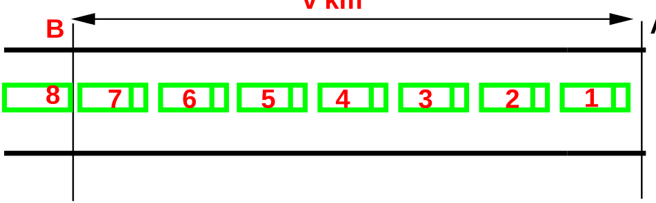
Let the number of vehicles counted by an observer at A for one hour be \(n_1\). By definition, the number of vehicles counted in one hour is flow(q). Therefore, \begin {equation} n_1 = q. \label {qe1} \end {equation}
Similarly, by definition, density is the number of vehicles in unit distance. Therefore number of vehicles \(n_2\) in a road stretch of distance \(v_1\) will be density \(\times \) distance.Therefore, \begin {equation} n_2 = k\times v. \label {qe2} \end {equation} Since all the vehicles have speed \(v\), the number of vehicles counted in 1 hour and the number of vehicles in the stretch of distance \(v\) will also be same.(ie \(n_1 = n_2\)). Therefore, \begin {equation} q = k\times v. \label {qe3} \end {equation} This is the fundamental equation of traffic flow. Please note that, \(v\) in the above equation refers to the space mean speed will also be same.
The relation between flow and density, density and speed, speed and flow, can be represented with the help of some curves. They are referred to as the fundamental diagrams of traffic flow. They will be explained in detail one by one below.
The flow and density varies with time and location. The relation between the density and the corresponding flow on a given stretch of road is referred to as one of the fundamental diagram of traffic flow. Some characteristics of an ideal flow-density relationship is listed below:
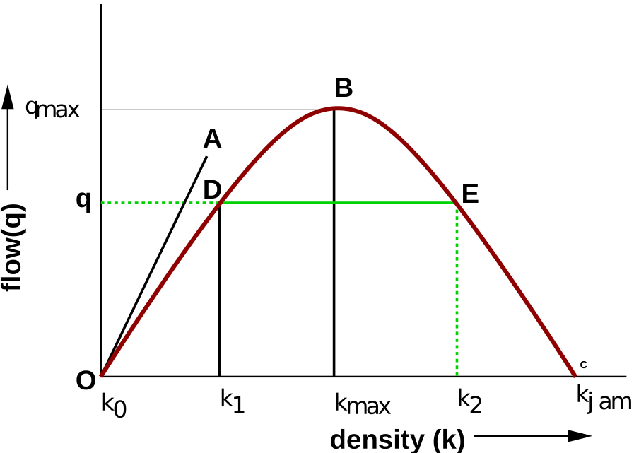
The point O refers to the case with zero density and zero flow. The point B refers to the maximum flow and the corresponding density is \(k_{max}\). The point C refers to the maximum density \(k_{jam}\) and the corresponding flow is zero. OA is the tangent drawn to the parabola at O, and the slope of the line OA gives the mean free flow speed, ie the speed with which a vehicle can travel when there is no flow. It can also be noted that points D and E correspond to same flow but has two different densities. Further, the slope of the line OD gives the mean speed at density \(k_1\) and slope of the line OE will give mean speed at density \(k_2\). Clearly the speed at density \(k_1\) will be higher since there are less number of vehicles on the road.
Similar to the flow-density relationship, speed will be maximum, referred to as the free flow speed, and when the density is maximum, the speed will be zero. The most simple assumption is that this variation of speed with density is linear as shown by the solid line in figure 4. Corresponding to the zero density, vehicles will be flowing with their desire speed, or free flow speed. When the density is jam density, the speed of the vehicles becomes zero.
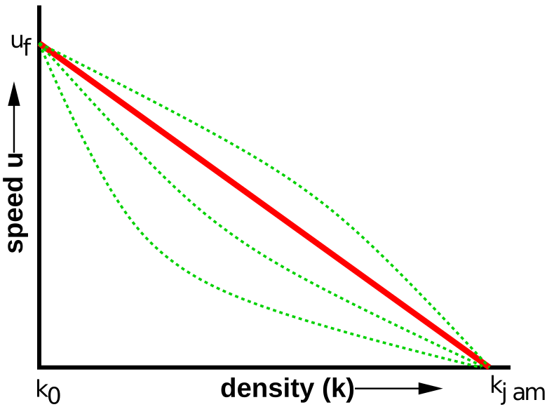
It is also possible to have non-linear relationships as shown by the dotted lines. These will be discussed later.
The relationship between the speed and flow can be postulated as follows. The flow is zero either because there is no vehicles or there are too many vehicles so that they cannot move. At maximum flow, the speed will be in between zero and free flow speed. This relationship is shown in figure 5.
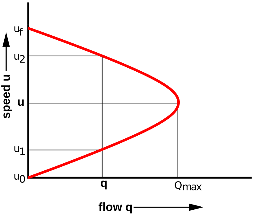
The maximum flow \(q_{max}\) occurs at speed \(u\). It is possible to have two different speeds for a given flow.
The diagrams shown in the relationship between speed-flow, speed-density, and flow-density are called the fundamental diagrams of traffic flow. These are as shown in figure 6. One could observe the inter-relationship of these diagrams.
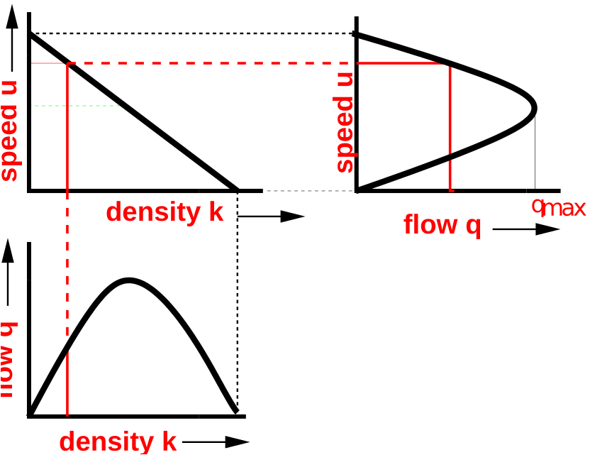
Time mean speed and space mean speed are two important measures of speed. It is possible to have a relation between them and was derived in this chapter. Also, time mean speed will be always greater than or equal to space mean speed. The fundamental diagrams of traffic flow are vital tools which enables analysis of fundamental relationships. There are three diagrams - speed-density, speed-flow and flow-density. They can be together combined in a single diagram as discussed in the last section of the chapter.
Calculate the time mean speed and the space mean speed of the following observation.
| Speed Range | Volume |
| (m/sec) | (veh/hr) |
| 10-12 | 12 |
| 12-14 | 18 |
| 14-16 | 24 |
| 16-18 | 20 |
| 18-20 | 14 |
The following travel times in seconds were measured for vehicles as they traversed a 3 km segmeny of a highway.
Compute the time mean speed and space mean speed for this data. Why space mean speed is always lower than time mean speed, explain with a derivation.
Calculate the time mean speed and the space mean speed of the following spot speed data:
| Speed Range | Volume |
| (m/sec) | (veh/hr) |
| 10-12 | 12 |
| 12-14 | 18 |
| 14-16 | 24 |
| 16-18 | 20 |
| 18-20 | 14 |
For the data given below,compute the time mean speed and space mean speed. Also verify the relationship between them. Finally compute the density of the stream.
| Speed range | Frequency |
| 1-4 | 5 |
| 5-8 | 15 |
| 9-12 | 23 |
| 13-16 | 24 |
| 17-20 | 16 |
I wish to thank several of my students and staff of NPTEL for their contribution in this lecture. I also appreciate your constructive feedback which may be sent to tvm@civil.iitb.ac.in. Prof. Tom V. Mathew, Department of Civil engineering, Indian Instiute of Technology Bombay, India.