Moving Observer Method

Lecture Notes in Transportation Systems Engineering

Prof. Tom V. Mathew

PDF for Online View or PDF for Print
(PDF for IITB students and is password protected)

1 Overview
2 Theory
3 Proof
4 Assumptions
4.0.1 Numerical Example 1
4.0.2 Numerical Example 2
5 Summary
Exercises
References
Acknowledgments

______________________________________________________________________

1 Overview

For a complete description of traffic stream modeling, one would require flow, speed, and density. Obtaining these parameters simultaneously is a difficult task if we use separate techniques. Since we have a fundamental equation of traffic flow, which gives the flow as the product of density and space mean speed, if we knew any two parameters, the third can be computed. Moving car or moving observer method of traffic stream measurement has been developed to provide simultaneous measurement of traffic stream variables. It has the advantage of obtaining the complete state with just three observers, and a vehicle. Determination of any of the two parameters of the traffic flow will provide the third one by the equation q = u.k. Thus, moving observer method is the most commonly used method to get the relationship between the fundamental stream characteristics. In this method, the observer moves in the traffic stream unlike all other previous methods.

2 Theory

Consider a stream of vehicles moving in the north bound direction. Two different cases of motion can be considered. The first case considers the traffic stream to be moving and the observer to be stationary.

Figure 1: Illustration of moving observer method

If n_o is the number of vehicles overtaking the observer during a period, t, then flow q is n0t , or

n = q × t 0

(1)

The second case assumes that the stream is stationary and the observer moves with speed v_o. If n_p is the number of vehicles overtaken by observer over a length l, then by definition, density k is npl- , or

np = k × l

(2)

n = k.v.t p o

(3)

where v₀ is the speed of the observer and t is the time taken for the observer to cover the road stretch. Now consider the case when the observer is moving within the stream. In that case m_o vehicles will overtake the observer and m_p vehicles will be overtaken by the observer in the test vehicle. Let the difference m is given by m₀ - m_p, then from equation 1 and equation 3,

m = m0 - mp = q t - k vo t

(4)

This equation is the basic equation of moving observer method, which relates q,k to the counts m, t and v_o that can be obtained from the test. However, we have two unknowns, q and k, but only one equation. For generating another equation, the test vehicle is run twice once with the traffic stream and another one against traffic stream, i.e.

mw = q tw - k vw tw (5) = q tw - k l ma = q ta + k va ta (6) = q ta + k l

where, a,w denotes against and with traffic flow. It may be noted that the sign of equation 6 is negative, because test vehicle moving in the opposite direction can be considered as a case when the test vehicle is moving in the stream with negative velocity. Further, in this case, all the vehicles will be overtaking, since it is moving with negative speed. In other words, when the test vehicle moves in the opposite direction, the observer simply counts the number of vehicles in the opposite direction. Adding equation 5 and 6, we will get the first parameter of the stream, namely the flow(q) as:

q = mw-+-ma- tw + ta

(7)

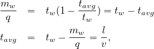
Now calculating space mean speed from equation 5,

mw- = q- kvw tw = q- qvw v [ ] = q- q l- v tw ( l -1 ) = q 1 - v × tw ( t ) = q 1 - avg- tw

If v_s is the mean stream speed, then average travel time is given by t_avg = vls

. Therefore,

mw- = tw(1- tavg) = tw - tavg q tw tavg = tw - mw-= l, q v

Rewriting the above equation, we get the second parameter of the traffic flow, namely the mean speed v_s and can be written as,

v = ---l---- s tw - mwq-

(8)

Thus two parameters of the stream can be determined. Knowing the two parameters the third parameter of traffic flow density (k) can be found out as

q k = v- s

(9)

For increase accuracy and reliability, the test is performed a number of times and the average results are to be taken.

3 Proof

4 Assumptions

4.0.1 Numerical Example 1

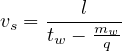
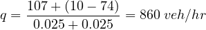
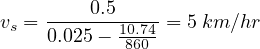
The length of a road stretch used for conducting the moving observer test is 0.5 km and the speed with which the test vehicle moved is 20 km/hr. Given that the number of vehicles encountered in the stream while the test vehicle was moving against the traffic stream is 107, number of vehicles that had overtaken the test vehicle is 10, and the number of vehicles overtaken by the test vehicle is 74, find the flow, density and average speed of the stream.

Solution

Time taken by the test vehicle to reach the other end of the stream while it is moving along with the traffic is t_w = = 0.025 hr
Time taken by the observer to reach the other end of the stream while it is moving against the traffic is t_a = t_w = 0.025 hr
Flow is computed from equation 7 as,
$q = 1007.0+2(51+00-.0 7245) = 860 veh∕hr$
Stream speed v_s is computed from equation 8 as
$v = ----0.5-----= 5 km∕hr s 0.025 - 108.6740-$
Density can be computed from the fundamental relation as
$k = qvs-= 8650 = 172 veh∕km$

4.0.2 Numerical Example 2

Table 1: Solution to the numerical example 2


No	m_a	m_o	m_p	m_w = (m_o - m_p)	t_a	t_w	q =	u =	k =

1	107	10	74	-64	0.025	0.025	860	5.03	171

2	113	25	41	-16	0.025	0.025	1940	15.04	129

3	30	15	5	10	0.025	0.025	800	40	20

4	79	18	9	9	0.025	0.025	1760	25.14	70

The data from four moving observer test methods are shown in the table. Column 1 gives the sample number, column 2 gives the number of vehicles moving against the stream, column 3 gives the number of vehicles that had overtaken the test vehicle, and last column gives the number of vehicles overtaken by the test vehicle. Find the three fundamental stream parameters for each set of data. Also plot the fundamental diagrams of traffic flow.


No	1	2	3

1	107	10	74

2	113	25	41

3	30	15	5

4	79	18	9

Solution From the calculated values of flow, density and speed, the three fundamental diagrams can be plotted as shown in figure 2.

Figure 2: Fundamental diagrams of traffic flow

5 Summary

Traffic engineering studies differ from other studies in the fact that they require extensive data from the field which cannot be exactly created in any laboratory. Speed data are collected from measurements at a point or over a short section or over an area. Traffic flow data are collected at a point. Moving observer method is one in which both speed and traffic flow data are obtained by a single experiment.

Exercises

Derive the expression for flow across a section of road by moving car method. Prove that this formulae actually estimates the stream flow.
In a traffic stream, 30% of the vehicles travel at a constant speed of 60km/h, 30% at a constant speed of 80km/h, and the remaining vehicles at a constant speed of 100km/h. An observer travelling at a constant speed of 70km/h with the stream over a length of 5km is overtaken by 17 vehicles more than what he has overtaken. The observer met 303 vehicles while traveling against the stream at the same speed and over the same length of highway. What is the mean speed and flow of the traffic stream?
Two friends were traveling from Mumbai to Pune and have decided to count the vehicles on a short stretch of 5 km. The first one sat on the left side and counted vehicles passed by him. The second sat on the right side and counted vehicles overtaken him. They counted 20 and 60 respectively while traveling at 30 kmph. They did the same exercise on the next day about same time and counted 25 and 40 respectively and were traveling at 35 kmph. Assuming same traffic conditions on both days, compute the density, mean speed, and flow on that stretch.
The observations from a moving car method are given in the table below. The column (1) shows the number of vehicles overtaken by the test vehicle, (2) show the number overtaking the test vehicle, (3) shows the number of vehicles moving against traffic stream, (4) is the travel time with the traffic (s), and (4) is the travel time against the traffic (s). Assuming linear speed-density relation, what is the maximum flow, speed, and density the following following stretch can take. Show the details of the calculation.

(1) (2) (3) (4) (5)
5 119 618 422 268
26 12 389 213 188
24 9 401 226 396
2 55 410 274 255
26 9 374 226 396
A moving vehicle experiment was conducted on a 2.5 km section of a highway. Two trials were conducted in the direction of dominant traffic flow. In the first trial, number of vehicles that had overtaken the test vehicle is 30, number of vehicles overtaken by the test vehicle is 6, and test vehicle speed is 30 kmph. In the second trial, number of vehicles that had overtaken the test vehicle is 20, number of vehicles overtaken by the test vehicle 26, and test vehicle speed is 35 kmph. Calculate the fundamental parameters of traffic flow and the average headway and spacing.
A person walking from office on a one-way street takes 60 min to get home, of which 12 min was taken talking to the driver of a stalled vehicle. He counted 52 vehicles while he was walking and 25 vehicles while he stopped. What are the travel time and flow of the vehicle stream?
A student riding his bicycle from campus on a one-way street takes 50 min to get home, of which 10 min was taken talking to the driver of a stalled vehicle. He counted 42 vehicles while he rode his bicycle and 35 vehicles while he stopped. What are the travel time and flow of the vehicle stream? (6)

References

L R Kadiyali. Traffic Engineering and Transportation Planning. Khanna Publishers, New Delhi, 1987.
C. S Papacostas. Fundamentals of Transportation Engineering. Prentice-Hall, New Delhi, 1987.

Web links

Acknowledgments

I wish to thank several of my students and staff of NPTEL for their contribution in this lecture. I also appreciate your constructive feedback which may be sent to tvm@civil.iitb.ac.in

Prof. Tom V. Mathew
Department of Civil Engineering
Indian Institute of Technology Bombay, India

_________________________________________________________________________

Monday 21 August 2023 12:19:24 AM IST


(1)	(2)	(3)	(4)	(5)

5	119	618	422	268

26	12	389	213	188

24	9	401	226	396

2	55	410	274	255

26	9	374	226	396


(1)	(2)	(3)	(4)	(5)

5	119	618	422	268

26	12	389	213	188

24	9	401	226	396

2	55	410	274	255

26	9	374	226	396