Contents

1 Introduction

The data required by a traffic engineer can mainly be observed on field rather than at laboratory. Now the field studies can be classified into three types depending upon the length of observation:

1. Measurement at a point
2. Measurement over a short section
3. Measurement over a long section

Out of these we will be discussing the first type here. Flow is the main traffic parameter measured at a point. Flow can be defined as the no of vehicles passing a section per unit time. Traffic volume studies are mainly carried out to obtain factual data concerning the movement of vehicles at selected point on the street or highway system.

2 Basic concepts

2.1 Types of Volume Measurement

Volume count varies considerably with time. Hence, several types of measurement of volume are commonly adopted to average these variations. These measurements are described below:

2.1.1 Average Annual Daily Traffic (AADT)

This is given by the total no. of vehicles passing through a section in a year divided by 365. This can be used for following purposes:

1. Measuring the present demand for service by the street or highway
2. Developing the major or arterial street
3. Evaluating the present traffic flow with respect to the street system
4. Locating areas where new facilities or improvements to existing facilities are needed.

2.1.2 Average Annual Weekday Traffic (AAWT)

This is defined as the average 24-hour traffic volume occurring on weekdays over a full year.

2.1.3 Average Daily Traffic (ADT)

An average 24-hour traffic volume at a given location for some period of time less than a year. It may be measured for six months, a season, a month, a week, or as little as two days. An ADT is a valid number only for the period over which it was measured.

2.1.4 Average Weekday Traffic (AWT)

An average 24-hour traffic volume occurring on weekdays for some period of time less than one year, such as for a month or a season.

2.2 Type of Counts

Various types of traffic counts are carried out, depending on the anticipated use of the data to be collected. They include:

2.2.1 Cordon Count

These are made at the perimeter of an enclosed area (CBD, shopping center etc.). Vehicles or persons entering and leaving the area during a specified time period are counted.

2.2.2 Screen Line Count

These are classified counts taken at all streets intersecting an imaginary line (screen line) bisecting the area. These counts are used to determine trends, expand urban travel data, traffic assignment etc.

2.2.3 Pedestrian Count

These are used in evaluating sidewalk and crosswalk needs, justifying pedestrian signals, traffic signal timings etc.

2.2.4 Intersection Count

These are measured at the intersections and are used in planning turn prohibitions, designing channelization, computing capacity, analyzing high accident intersections etc.

2.3 Counting Techniques

Number of vehicles can be counted either manually or by machine depending upon the duration of study, accuracy required, location of study area etc.

2.3.1 Manual counting

In its simplest form an observer counts the numbers of vehicles along with its type, passing through the section for a definite time interval. For light volumes, tally marks on a form are adequate. Mechanical or electrical counters are used for heavy traffic. Although it is good to take some manual observations for every counting for checking the instruments, some other specific uses of manual counts are following:

1. Turning and through movement studies
2. Classification and occupancy studies
3. For analysis of crosswalks, sidewalks, street corner space and other pedestrian facilities

2.3.2 Automatic counting

These can be used to obtain vehicular counts at non-intersection points. Total volume, directional volume or lane volumes can be obtained depending upon the equipment available.

2.3.3 Permanent Counters

These are installed to obtain control counts on a continuous basis. A detector (sensor) which responds on the passage of vehicle past a selected point is an essential part of this type of counters. These can be mainly grouped into contact types, pulsed types, radar types. Among the contact type counters, pneumatic tubes are mostly used. Air pulse actuated by vehicle wheels, pass along the tube thereby increasing the count. Pulsed types mainly depend upon the interruption of a beam generated from a station located near the site, which is detected by the receiver. In radar types, a continuous beam of energy is directed towards the vehicle. The frequency shift of energy reflected from approaching vehicle is conceived by sensors. Due to tedious reduction of the voluminous amount of data obtained, use of such counters was decreasing. But the use of computers and data readable counters has reversed the trend.

2.3.4 Portable Counters

These are used to obtain temporary or short term counts. Generally these make use of a transducer unit actuated by energy pulses. Each axle or vehicle passage operates a switch attached to a counter which is usually set to register one unit for every two axles. If significant number of multi-axle vehicles is present, an error is introduced. A correction factor, obtained from a sample classification count, is introduced to reduce this error. This can further be sub-divided into two types:

1. Recording counters provides a permanent record of volumes by printing the total volume. These may be set for various counting intervals.
2. Non-Recording Counters must be read by an observer at desired intervals.

2.4 Counting Periods

The time and length that a specific location should be counted depends upon the data desired and the application in which the data are used. Counting periods vary from short counts at spot points to continuous counts at permanent stations. Hourly counts are generally significant in all engineering design, while daily and annual traffic is important in economic calculations, road system classification and investment programmes. Continuous counts are made to establish national and local highway use, trends of use and behaviour and for estimating purposes. Some of the more commonly used intervals are:

1. 24-hour counts normally covering any 24-hour period between noon Monday and noon Friday. If a specific day count is desired, the count should be from midnight to midnight.
2. 16 hour counts usually 5:30 am to 9:30 pm or 6 am to 9 pm.
3. 12 hour counts usually from 7 am to 7 pm
4. Peak Period counting times vary depending upon size of metropolitan area, proximity to major generators and the type of facility. Commonly used periods are 7 to 9 am and 4 to 6 pm.

3 Variation of Volume Counts and Peak Hour Factors

Variation of volume counts can be further sub-divided into daily, weekly and seasonal variation. For studying the daily variation, the flow in each hour has been expressed as percentage of daily flow. Weekdays, Saturdays and Sundays usually show different patterns. That’s why comparing day with day is much more useful. Peak Hour Volume is very important factor in the design of roads and control of traffic, and is usually 2 - 2.5 times the average hourly volume. Apart from this there is one additional feature of this variation: two dominant peaks (morning and evening peak), especially in urban areas. These mainly include work trips and are not dependent on weather and other travel conditions.

Similar to daily variation, weekly variation gives volumes expressed as a percentage of total flow for the week. Weekdays flows are approximately constant but the weekend flows vary a lot depending upon the season, weather and socio-economic factors. Seasonal variation is the most consistent of all variation patterns and represents the economic and social condition of the area served.

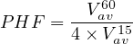
Peak hour factors should be applied in most capacity analyses in accordance with the Highway Capacity Manual, which selected 15 minute flow rates as the basis for most of its procedures. The peak-hour factor (PHF) is descriptive of trip generation patterns and may apply to an area or portion of a street and highway system. The PHF is typically calculated from traffic counts. It is the average volume during the peak 60 minute period V _av⁶⁰ divided by four times the average volume during the peak 15 minute’s period V _av¹⁵.

(1)

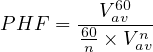
One can also use 5, 10, or 20 minutes instead of 15 minutes interval for the calculation of PHF. But in that case we have to change the multiplying factor in the denominator from 4. Generalizing,

(2)

where V _avⁿ is the peak n minute flow. The Highway Capacity Manual advises that in absence of field measurements reasonable approximations for peak hour factor can be made as follows:

1. 0.95 for congested condition
2. 0.92 for urban areas
3. 0.88 for rural areas

General guidelines for finding future PHF can be found in the Development Review Guidelines, which are as follows:

1. 0.85 for minor street inflows and outflows
2. 0.90 for minor arterial
3. 0.95 for major streets

3.0.1 Numerical Example

The table below shows the volumetric data observed at an intersection. Calculate the peak hour volume, peak hour factor (PHF), and the actual (design) flow rate for this approach.

Solution We can locate the hour with the highest volume and the 15 minute interval with the highest volume. The peak hour is shown in blue below with the peak 15 minute period shown in bold font.

The peak hour volume is just the sum of the volumes of the four 15 minute intervals within the peak hour (219). The peak 15 minute volume is 65 in this case. The peak hour factor (PHF) is found by dividing the peak hour volume by four times the peak 15 minute volume. PHF = = 0.84 The actual (design) flow rate can be calculated by dividing the peak hour volume by the PHF, 219/0.84 = 260 vehicles/hr, or by multiplying the peak 15 minute volume by four, 4 × 65 = 260 vehicles per hour.

4 Passenger Car Unit (PCU)

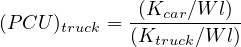
Passenger Car Unit (PCU) is a metric used in Transportation Engineering, to assess traffic-flow rate on a highway. A Passenger Car Unit is a measure of the impact that a mode of transport has on traffic variables (such as headway, speed, density) compared to a single standard passenger car. This is also known as passenger car equivalent. For example, typical values of PCU (or PCE) are:

Highway capacity is measured in PCU/hour daily.

4.0.1 Numerical Example

The table below shows the volumetric data collected at an intersection: Calculate the peak hour volume, peak hour factor (PHF), and the actual (design) flow rate for this approach.

Solution The first step in this solution is to find the total traffic volume for each 15 minute period in terms of passenger car units. For this purpose the PCU values given in the table are used. Once we have this, we can locate the hour with the highest volume and the 15 minute interval with the highest volume. The peak hour is shown in blue below with the peak 15 minute period shown in a darker shade of blue.

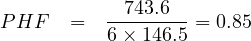
The peak hour volume is just the sum of the volumes of the six 10 minute intervals within the peak hour (743.6 PCU). The peak 10 minute volume is 146.5 PCU in this case. The peak hour factor (PHF) is found by dividing the peak hour volume by four times the peak 10 minute volume.

5 Determination of PCU

Traffic in many parts of the world is heterogeneous, where road space is shared among many traffic modes with different physical dimensions. Loose lane discipline prevails; car following is not the norm. This complicates computing of PCU. Some of the methods for determining passenger car units (PCU) are following:

1. Modified Density Method
2. Chandra’s method
3. Method Based on Relative Delay
4. Headway method
5. Multiple linear regression method
6. Simulation method

It may be appropriate to use different values for the same vehicle type according to circumstances like volume of traffic, speed of vehicle, lane width and several external factors.

5.1 Method based on relative delay

The 1965 HCM used relative speed reduction to define PCUs for two lane highways and quantified this by the relative number of passing known as the Walker method. For multi-lane highways, PCUs were based on the relative delay due to trucks. PCUs for multi-lane highways based on relative delay may be found as

(3)

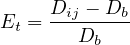
where D_ij is the delay to passenger cars due to vehicle type i under condition j and D_b is the base delay to standard passenger cars due to slower passenger cars.

PCUs in the 1965 HCM were reported for grades of specific length and percent, proportion of trucks, and LOS grouped as A through C or D and E. As expected, the highest PCU was reported for the longest and steepest grade with the highest proportion of trucks and the lowest LOS. However, in many cases the PCU for a given grade and LOS decreased with increasing proportion of trucks. PCUs in the 1965 HCM were reported for grades of specific length and percent, proportion of trucks, and LOS grouped as A through C or D and E. As expected, the highest PCU was reported for the longest and steepest grade with the highest proportion of trucks and the lowest LOS. However, in many cases the PCU for a given grade and LOS decreased with increasing proportion of trucks.

5.2 Multiple linear regression model

Multiple linear regression method try to represent the speed of a traffic stream as function of number of variables. For example, the percentile speed v_p can represented as:

(4)

where v_f is the free speed, V _c is the number of passenger cars, V _c is the number of trucks V _r is the number of recreational vehicles, V _r is the number of other types of vehicles, V _a is the number of vehicles moving against the current stream, C₁ to C₅ are coefficient representing the relative sizes of speed reductions for each vehicle type. Although this model was formulated for two lane highways with opposing traffic flow, it could be applied to multi-lane highways by setting the coefficient C₅ to zero. Using the speed reduction coefficients, E_n, the PCU for a vehicle type n is calculated as:

where C_n is the speed reduction coefficient for vehicle type n and C₁ is the speed reduction coefficient for passenger cars.

5.3 Method based on headway

Realizing one of the primary effects of heavy vehicles in the traffic stream is that they take up more space, headways have been used for some of the most popular methods to calculate PCUs. In 1976, Werner and Morrall suggested that the headway method is best suited to determine PCUs on level terrain at low levels of service. The PCU is calculated as

(5)

where H_M is the average headway for a sample including all vehicle types, H_B is the average headway for a sample of passenger cars only, P_C is the proportion of cars, and P_T is the proportion of trucks.

5.3.1 Numerical Example

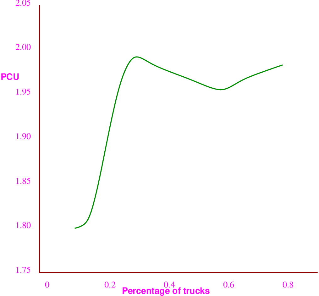
The table given below show headway data for a number of traffic conditions. It is assumed that the traffic contains only car and truck. Compute the PCU value for each traffic condition Note that h_m, h_c, p_c, p_t respectively denote the average headway for mixed traffic, average headway for traffic consisting of cars only, the percentage of cars and percentage of trucks of the traffic stream.

Solution Use the formula given above to find the value of PCU.

5.4 Chandra’s method

This method uses two factors: namely, velocity of vehicle type and its projected rectangular area to calculate the PCU value.

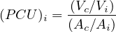(6)

where V _c and V _i are mean speeds of car and vehicle of type i respectively and A_c and A_i are their respective projected rectangular area  length * width on the road.

5.4.1 Numerical Example

The table given shows the data obtained in spot speed study for various vehicle types. Find the PCU value for each vehicle type using the Chandra’s Method.

Solution Step 1 We have to find the space mean speed for each vehicle type using the formula:

Step 2 Find the PCU values using Chandra’s Method. Use the table having the areas of various vehicle types given above.

Then we can use the table given above to find the areas of different vehicle types to find corresponding PCU values.

5.5 Density method

In the density method, the PCU of truck (E_t) is computed as:

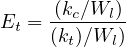(7)

where k_c is the density of cars in pure homogeneous conditions(car/km.), W_l is the width of the lane in homogeneous traffic, k_t is the density of the truck in pure homogeneous conditions and E_t is the passenger car unit of the trucks given homogeneous traffic behaviour. In density method where car following and lane discipline behaviour prevails, all traffic entities use an equal W_l.

5.5.1 Numerical Example

The table given below shows the data of flow and space mean speed of Car and HCV in a two lane road without shoulders. Assume the 85 percentile distribution width of HCV and Car to be 9.50m. and 7.50m. Compute the PCU value of HCV for each time interval.

Solution We know that PCU value can be calculated using the formula:

(8)

Step 1 Find the density of car and truck using basic relationship between the traffic flow parameters

(9)

Step 2 The using the method stated above we can find the PCU values. The table showing the PCU values has been illustrated below.

6 Conclusion

Measurement over a section is probably one of the easiest field parameter that can be measured. Various types of volume counts and counting techniques have been discussed in brief. Along with this a brief insight into various methods of calculating Passenger Car unit has been provided. Out of the various methods discussed, Chandra’s Method is only method that can be applied to the Indian condition of heterogeneous traffic that is characterized by loose lane discipline. All the other methods are primarily based on homogeneous traffic conditions mainly prevailing in developed countries.

Exercises

1. The table below shows spot speed data (in meters/sec) and the projected area (PA) of each vehicle type (in square meters) from a study. Find the PCU value of each vehicle type using Chandra’s method.

   No	Car	3W	2W	HCV
   PA	5.39	4.48	1.20	24.74
   1	11.32	8.67	6.67	7.4
   2	6.74	7.25	8.27	6.09
   3	11.11	9.68	7.75	5.88
   4	6.67	6.98	6.12	6.38
   5	8.11	8.77	9.52	5.66
   6	7.41	8.77	11.9	5.66
   7	8.11	9.52	6.97	5.55

2. Cars, bikes, auto-rickshaws, and buses are moving in a traffic stream with means speeds of 10, 9, 8, and 7 m/sec. Further, the proportion of these vehicles among the 3000 vehicles counted in an hour is found to be 40, 30, 20, 10 per cent respectively. Compute the flow rate in passenger car units if the equivalency concept proposed by Chandra is adopted. Make suitable assumptions if required.

References

1. S Chandra and U Kumar. Effect of lane width on capacity under mixed traffic conditions in india. Journal of Transportation Engineering, ASCE, 129:155–160, 2003.
2. F D Hobbs. Traffic Planning and Engineering. Pergamon Press, 1979. 2nd Edition.
3. W S Homburger. Fundamentals of traffic engineering. 2019. 12th Edition, pp 5-1 to 5-5.
4. Anthony Ingle. Development of Passenger Car Equivalents for Basic Freeway Segments. Blacksburg, Virginia, July 8, 2004.
5. Geetam Tiwari, Joseph Fazio, and Sri Pavitravas. Passenger Car Units for Heterogeneous Traffic Using a Modified Density Method. 2019.

Acknowledgments

I wish to thank several of my students and staff of NPTEL for their contribution in this lecture. I also appreciate your constructive feedback which may be sent to tvm@civil.iitb.ac.in

Prof. Tom V. Mathew
Department of Civil Engineering
Indian Institute of Technology Bombay, India