Contents

1 Overview

The main purpose of this chapter is to determine traffic parameter, specially speed. Speed measurements are most often taken at a point (or a short section) of road way under conditions of free flow. The intent is to determine the speeds that drivers select, unaffected by the existence of congestion. This information is used to determine general speed trends, to help determine reasonable speed limits, and to assess safety.

2 Speed Studies

As speed defines the distance travelled by user in a given time, and this is a vibrant in every traffic movement. In other words speed of movement is the ratio of distance travelled to time of travel. The actual speed of traffic flow over a given route may fluctuated widely, as because at each time the volume of traffic varies. Accordingly, speeds are generally classified into three main categories

1. Spot speed This is the instantaneous speed of a vehicle at any specific location.
2. Running speed This is the average speed maintained over a particular course while the vehicle is in the motion.
3. Journey speed This is the effective speed of the vehicle on a journey between two points and the distance between two points and the distance between these points divided by the total time taken for the vehicle to complete the journey, it includes all delay.

3 Spot Speed Studies

When we measure the traffic parameter over a short distance, we generally measure the spot speed. A spot speed is made by measuring the individual speeds of a sample of the vehicle passing a given spot on a street or highway. Spot speed studies are used to determine the speed distribution of a traffic stream at a specific location. The data gathered in spot speed studies are used to determine vehicle speed percentiles, which are useful in making many speed-related decisions. Spot speed data have a number of safety applications, including the following

1. Speed trends,
2. Traffic control planning,
3. Accidental analysis,
4. Geometric design,
5. Research studies.

4 Methods of Measurement

Methods of conducting spot speed Studies are divided into two main categories: Manual and Automatic. Spot speeds may be estimated by manually measuring the time it takes a vehicle to travel between two defined points on the roadway a known distance apart (short distance), usually less than 90m. Distance between two points is generally depending upon the average speed of traffic stream. Following tables gives recommended study length (in meters) for various average stream speed ranges (in kmph)

Following are the some methods to measure spot speed of vehicles in a traffic stream, in which first two are manual methods and other are automatic:

4.1 Pavement markings

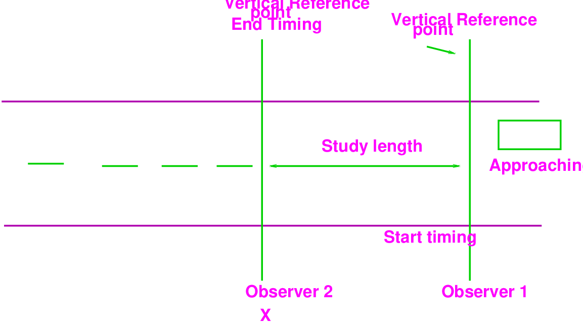
In this method, markings of pavement are placed across the road at each end of trap. Observer start and stops the watch as vehicle passes lines. In this method, minimum two observers required to collect the data, of which one is stand at the starting point to start and stop the stop watch and other one is stand at end point to give indication to stop the watch when vehicle passes the end line. Advantages of this method are that after the initial installation no set-up time is required, markings are easily renewed, and disadvantage of this is that substantial error can be introduced, and magnitude of error may change for substitute studies and this method is only applicable for low traffic conditions.

4.2 Enoscope or Mirror box

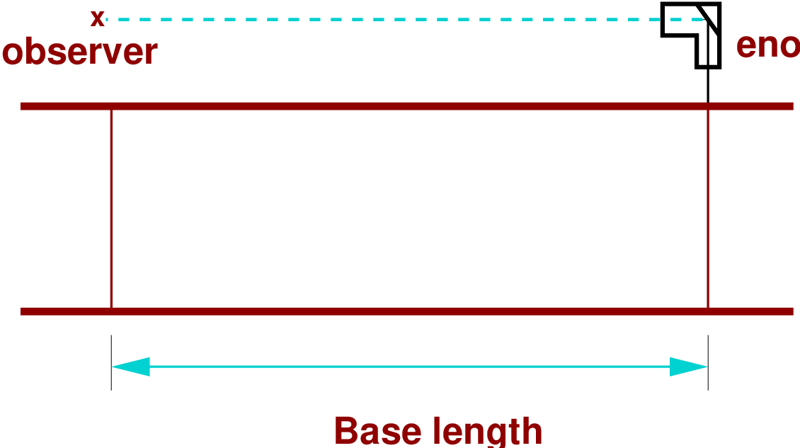
Enoscope consists of a simple open housing containing a mirror mounted on a tripod at the side of the road in such a way that an observer’s line of sight turned through 90o. The observer stands at one end of section and on the other end enoscope is placed and measure the time taken by the vehicle to cross the section (fig 6.2). Advantages of this method are that it simple and eliminate the errors due to parallax and considerable time is required to time each vehicle, which lengthen the study period and under heavy traffic condition it may be difficult to relate ostentatious to proper vehicle are the disadvantages of enoscope method.

4.3 Road Detector (Pressure contact strips)

Pressure contact strips, either pneumatic or electric, can be used to avoid error due to parallax and due to manually starting and stopping the chronometer or stopwatch. This is the best method over short distance it gives quite relevant data and if it is connected through graphical recorder then it gives continuous data automatically.

4.4 Doppler-Principle Meters (Radar)

This is recently developed method, it automatically records speed, employs a radar transmitter-receiver unit. The apparatus transmits high frequency electromagnetic waves in a narrow beam towards the moving vehicle, and reflected waves changed their length depending up on the vehicles speed and returned to the receiving unit, through calibration gives directly spot speed of the vehicle.

4.5 Electronic-Principle Detectors (Photography)

In this method a camera records the distance moved by a vehicle in a selected short time. In this exposure of photograph should be in a constant time interval and the distance travelled by the vehicle is measured by projecting the films during the exposure interval. The main advantage of method that, it gives a permanent record with 100% sample obtained. This method is quite expensive and generally used in developed cities. In this we can use video recorder which give more accurate result.

5 Data Collection Sheets

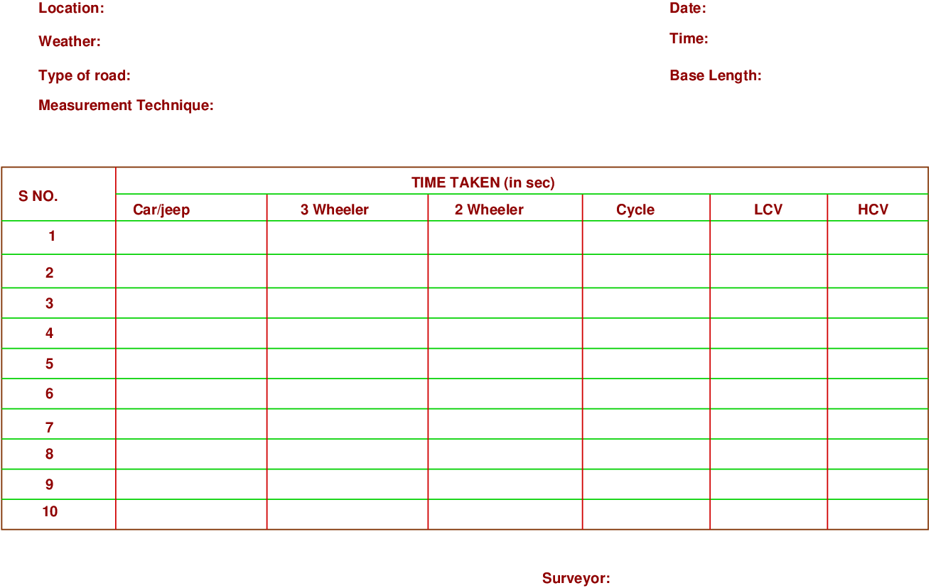
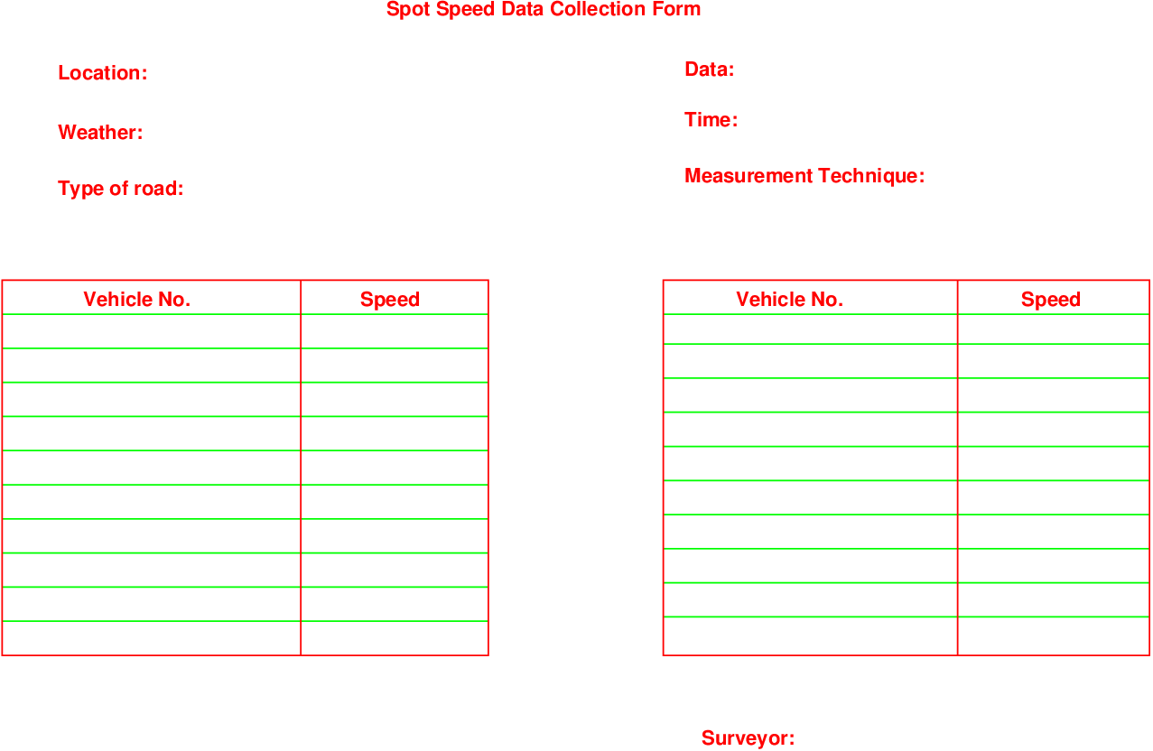
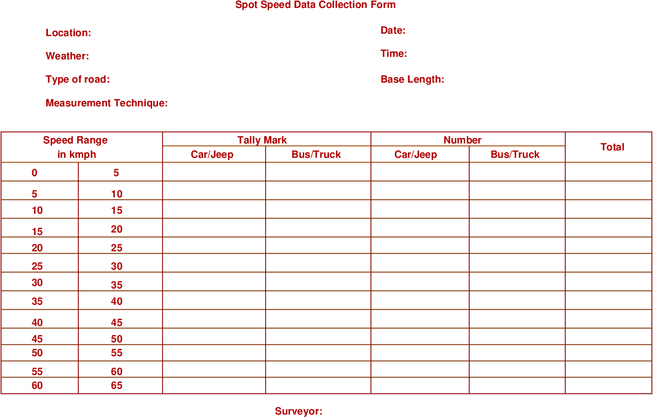
The measured data by the above techniques should be collected into some formats, following are the some types of data collection sheets which are used for manual and automatic methods,

1. For Enoscope and Pavement Marking Methods

   ---

   
   

   Figure 3: Data collection sheet for Enoscope and Pavement Marking Methods

   ---

2. For automatic methods

   ---

   
   

   Figure 4: Data collection sheet for Automatic Methods

   ---

   ---

   
   

   Figure 5: Data collection sheet for Automatic Methods

   ---

6 Data Presentation

From the above methods, the collected data have to present into the some representable form, this makes its calculation and analysis simpler and easier. The following methods to present the spot speed data:

6.1 Frequency Distribution Table

After the collection of data in the given conditions, arrange the spot speed values in order to their magnitudes. Then select an interval speed (e.g. 5 kmph) and make grouping of data which come under this range. Now, prepare the frequency distribution table.

6.2 Frequency Distribution Curve

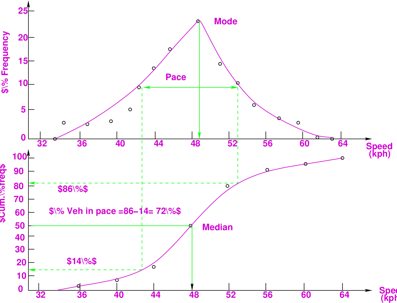
For each speed group, the % frequency of observations within the group is plotted versus the middle (mid-mark) speed of the group(s). As shown in Fig 6.5. From this curve the modal speed and pace of traffic flow can be determine. Generally the shape of the curve follows the normal distribution curve, this because the most of the vehicles move on road near by mean speed and very few deviate from mean speed.

6.3 Cumulative Frequency Distribution Curve

For each speed group, the % cumulative frequency of observations is plotted versus the higher limit of the speed group (Fig 6.5). The cumulative frequency distribution curve, however, results in a very useful plot of speed versus the percent of vehicles traveling at or below the designated speed. For this reason, the upper limit of the speed group is used as the plotting point. In both the distribution curve, the plots are connected by a smooth curve that minimizes the total distance of points falling above the line and those falling below the line. A smooth curve is defined as one without.

7 Distribution Characteristics

Common descriptive statistics may be computed from the data in the frequency distribution table or determined graphically from the frequency and cumulative frequency distribution curves. These statistics are used to describe two important characteristics of the distribution:

7.1 Measure of Central Tendency

Measure which helps to describe the approximate middle or center of the distribution. Measures of central tendency include the average or mean speed, the median speed, the modal speed, and the pace.

7.1.1 Mean Speed

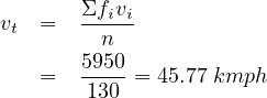
The arithmetic (or harmonic) average speed is the most frequently used speed statistics. It is the measure of central tendency of the data. Mean calculated gives two kinds of mean speeds.

(1)

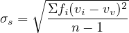
where, v_t is the mean or average speed, v_i is the individual speed of the i_th vehicle, f_i is the frequency of speed, and n is the total no of vehicle observed (sample size). Time mean Speed If data collected at a point over a period of time, e.g. by radar meter or stopwatch, produce speed distribution over time, so the mean of speed is time mean speed. Space mean Speed If data obtained over a stretch (section) of road almost instantaneously, aerial photography or enoscope, result in speed distribution in space and mean is space mean speed. Distribution over space and time are not same. Time mean speed is higher than the space mean speed. The spot speed sample at one end taken over a finite period of time will tend to include some fast vehicles which had not yet entered the section at the start of the survey, but will exclude some of the slower vehicles. The relationship between the two mean speeds is expressed by:

(2)

where, v_t and v_s are the time mean speed and space mean speed respectively. And σ_s is the standard deviation of distribution space.

7.1.2 Median Speed

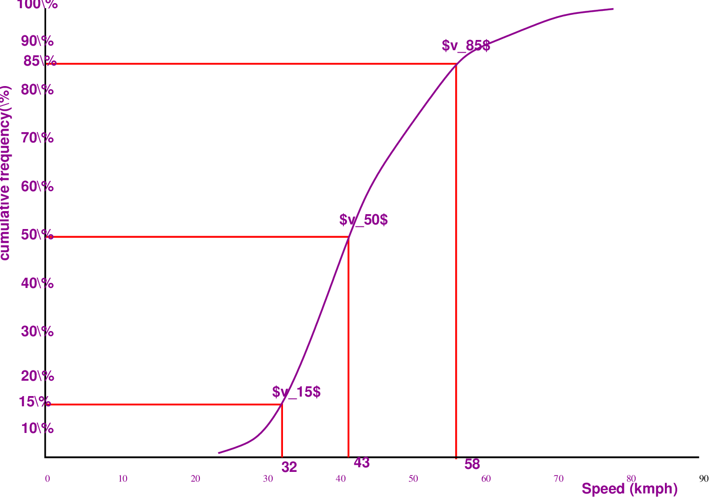
The median speed is defined as the speed that divides the distribution in to equal parts (i.e., there are as many observations of speeds higher than the median as there are lower than the median). It is a positional value and is not affected by the absolute value of extreme observations. By definition, the median equally divides the distribution. Therefore, 50% of all observed speeds should be less than the median. In the cumulative frequency curve, the 50th percentile speed is the median of the speed distribution. Median Speed = v50

7.1.3 Pace

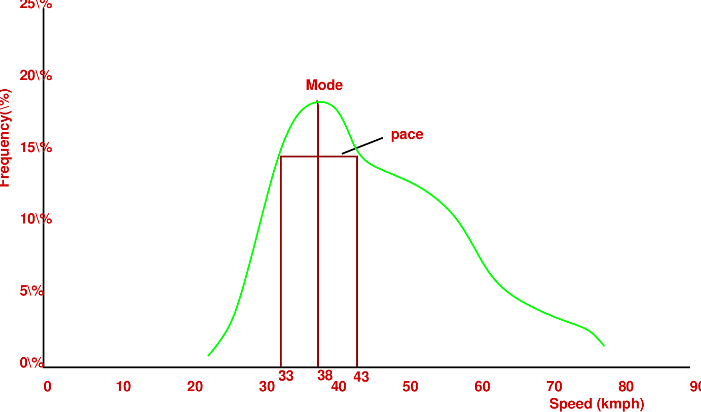
The pace is a traffic engineering measure not commonly used for other statistical analyses. It is defined as the 10Km/h increment in speed in which the highest percentage of drivers is observed. It is also found graphically using the frequency distribution curve. As shown in fig 6.5. The pace is found as follows: A 10 Km/h template is scaled from the horizontal axis. Keeping this template horizontal, place an end on the lower left side of the curve and move slowly along the curve. When the right side of the template intersects the right side of the curve, the pace has been located. This procedure identifies the 10 Km/h increments that intersect the peak of the curve; this contains the most area and, therefore, the highest percentage of vehicles.

7.1.4 Modal Speed

The mode is defined as the single value of speed that is most likely to occur. As no discrete values were recorded, the modal speed is also determined graphically from the frequency distribution curve. A vertical line is dropped from the peak of the curve, with the result found on the horizontal axis.

7.2 Measure of Dispersion

Measures describe the extent to which data spreads around the center of the distribution. Measures of dispersion include the different percentile speeds i.e. 15th, 85th,etc. and the standard deviation.

7.2.1 Standard Deviation

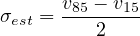
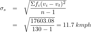
The most common statistical measure of dispersion in a distribution is the standard deviation. It is a measure of how far data spreads around the mean value. In simple terms, the standard deviation is the average value of the difference between individual observations and the average value of those observations. The Standard deviation, σ_s, of the sample can be calculated by

(3)

7.2.2 Percentile Speeds

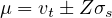
The 85th and 15th percentile speeds give a general description of the high and low speeds observed by most reasonable drivers. It is generally thought that the upper and lower 15% of the distribution represents speeds that are either too fast or too slow for existing conditions. These values are found graphically from the cumulative frequency distribution curve of Figure 6.4. The curve is entered on the vertical axis at values of 85% and 15%. The respective speeds are found on the horizontal axis. The 85th and 15th percentile speeds can be used to roughly estimate the standard deviation of the distribution σ_est, although this is not recommended when the data is available for a precise determination.

(4)

The 85th and 15th percentile speeds give insight to both the central tendency and dispersion of the distribution. As these values get closer to the mean, less dispersion exists and the stronger the central tendency of the distribution becomes.

The 98th percentile speed is also determining from the cumulative frequency curve, this speed is generally used for geometric design of the road.

8 Data Analysis

8.1 Standard Error of the mean

The means of different sample taken from the same population are distributed normally about the true mean of population with a standard deviation, is known as standard error.

(5)

8.2 Sample Size

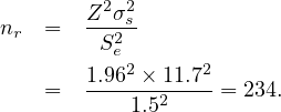
Generally, sample sizes of 50 to 200 vehicles are taken. In that case, standard error of mean is usually under the acceptable limit. If precision is prior then minimum no. of sample should be taken, that can be measured by using the following equation.

(6)

where, n_r is the no. of sample required, σ_s is the Standard deviation, Z is value calculated from Standard Normal distribution Table for a particular confidence level (i.e. for 95% confidence Z=1.96 and for 99.7% confidence Z=3.0) and Se is the permissible (acceptable) error in mean calculation.

8.3 Precision and Confidence Intervals

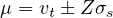
Confidence intervals express the range within which a result for the whole population would occur for a particular proportion of times an experiment or test was repeated among a sample of the population. Confidence interval is a standard way of articulate the statistical accuracy of an experiment based assessment. If assess has a high error level, the equivalent confidence interval will be ample, and the less confidence we can have that the experiment results depict the situation among the whole population. When quoting confidence It is common to refer to the some confidence interval around an experiment assessment or test result. So, the confidence interval for estimated true mean speed can be calculated by

(7)

where, μ is the confidence interval, v_t is mean speed, σ_s is standard deviation and Z is constant for specified confidence.

8.4 Numerical Example

Using the spot speed data given in the following table, collected from a freeway site operating under free-flow conditions: (i) Plot the frequency and cumulative frequency curves for these data; (ii) Obtain median speed, modal speed, pace, and percent vehicles in pace from these plots; (iii) Compute the mean and standard deviation of the speed distribution; (iv) The confidence bounds on the estimate of the true mean speed of the underlying distribution with 95% confidence? With 99.7% confidence; and (v) Based on these results, compute the sample size needed to achieve a tolerance of ±1.5 kmph with 95% confidence.

Solution For the spot speed study, first draw a frequency distribution table show below.

1. From the table 6.3, we can draw frequency distribution and cumulative frequency distribution curve.(shown in Fig 6.6 and 6.7)
   

   ---

   Range	V i	fi	%fi	%∑ fi	fiV i	fi(V i - V m)2
   21-25	23	2	2%	2%	46	1036.9
   26-30	28	6	5%	6%	168	1894.5
   31-35	33	18	14%	20%	594	2935.0
   36-40	38	25	19%	39%	950	1509.0
   41-45	43	19	15%	54%	817	145.7
   46-50	48	16	12%	66%	768	79.6
   51-55	53	17	13%	79%	901	888.8
   56-60	58	12	9%	88%	696	1795.1
   61-65	63	7	5%	94%	441	2078.3
   66-70	68	4	3%	97%	272	1976.8
   71-75	73	3	2%	99%	219	2224.5
   76-80	78	1	1%	100%	78	1038.8
   Total		130	100%		5950	17603.0

   
   

   Table 1: Solution of the example problem

   ---

2. From the curves, Median speed, v₅₀ = 43 kmph; Modal speed, = 38 kmph; the Pace = 33 - 43 kmph; Percent vehicles in pace = 54-20= 34%; and the 85th Percentile speed = 58 kmph.

   ---

   
   

   Figure 7: Frequency Distribution Curve

   ---

   ---

   
   

   Figure 8: Cumulative Frequency Distribution Curve

   ---

3. Mean is calculated by using
   
   Standard Deviation of the Speed
   
4. The confidence bounds on the estimate of the true mean speed of the underlying distribution are:
   1. For 95% confidence, Z= 1.96, so

   2. For 99.7% confidence, Z= 3.0, so

5. Sample size required for 95% confidence with acceptable error of 1.5 kmph
   
   So, given sample size is not sufficient and we require minimum 234 samples to achieve that confidence with given acceptable error. The results are summaries in table 8.4

9 Location for Speed Studies

The speed studies are accompanied for eminently logical purposes that will influence what traffic engineering measures are implemented in any given case. The location at which speed measurements are taken must conform to the intentional purpose of the study. The guiding philosophy behind spot speed studies is that measurements should include drivers freely selecting their speeds, unaffected by traffic congestion. For example if driver approaches to a toll plaza, then he has to slow his speed, so this is not suitable location to conduct the study, measurements should be taken at a point before drivers start to decelerate. Similarly, if excessive speed around a curve is thought to be contributing to off-the-road accidents, speed measurements should be taken in advance of the curve, before deceleration begins. It may also be appropriate, however, to measure speeds at the point where accidents are occurring for evaluation with approach speeds. This would allow the traffic engineer to assess whether the problem is excessive approach speed or that drivers are not decelerating sufficiently through the subject geometric element, or a combination of both. A study of intersection approach speeds must also be taken at a point before drivers begin to decelerate. This may be a moving point, given that queues get shorter and longer at different periods of the day.

10 Summary

This chapter has presented the basic concepts of speed studies. Spot speed studies are conducted to estimate the distribution of speeds of vehicle in the traffic stream at a particular position on highway. This is done by recording the speeds of vehicle at the specified location. These data are used to obtain speed characteristics such as mean speed, modal speed, pace, standard deviation and different percentile of speeds. The important factors which should consider during plan of studies is the location of study, time and duration of study. The data sample collected should contain samples size. These gives precision and accuracy of result.

Exercises

1. Determine the time mean speed, space mean speed, and 85^th percentile speed from the following speed (in m/s) data.

   Speed	Frequency
   1- 5	9
   6-10	16
   11-15	32
   16-20	48
   21-25	23
   26-30	9

2. For a given road following speed data is collected. 25, 31, 36, 39, 42, 44, 47, 48, 49, 51, 52, 52, 53, 54, 55, 56, 57, 57, 57, 58, 59, 60, 60, 62, 63, 64, 65, 66, 66, 68, 68, 69, 70, 70, 71, 73, 75, 79, 85, 89, 90. What is the speed you will recommend for designing sight distance or radius of circular curve?
3. The spot speeds of ten vehicles observed at a certain location are 55.1, 40.8, 32.2, 47.8, 64.5, 53.2, 58.2, 67.6, 36.4, and 53.2 kmph. Find the time mean speed, space mean speed and 85th percentile speed
4. Tabel below indicates the values of spot speeds observed at a certain location. Find (i) the 85th percentile speed and (ii) the probability that the speed exceeds 85th percentile assuming that speeds follow a normal distribution.

   Obs. No	Speed (kmph)
   1	55.1
   2	40.8
   3	32.2
   4	47.8
   5	64.5
   6	53.2
   7	58.2
   8	66.6
   9	36.4
   10	53.2

5. For the speed data given in Table below, what is the probability that the speed is greater than 25 kmph but less than 45 kmph? Assume suitable distribution for speed.

   Speed Range (kmph)		Observed
   Lower	Upper	Proportion
   Bound	Bound
   10	20	0.012
   20	30	0.178
   30	40	0.316
   40	50	0.218
   50	60	0.108
   60	70	0.055
   70	80	0.033
   80	90	0.022
   90	100	0.013
   100	110	0.045
   Number of observations		2600
   Mean speed in kmph		40
   Standard deviation		22
   Minimum possible speed		10

References

1. F D Hobbs. Traffic Planning and Engineering. Pergamon Press, 1979. 2nd Edition.
2. Nicholas J Garber Lester A Hoe. Traffic and Highway Engineering. Cengage Learning Product, Fourth Edition, 2009.
3. Theodore M Matson, Wilbur S Smith, and Frederick W Hurd. Traffic Engineering. McGraw Hill Book Company, New York, 1955.
4. R P Roess, S E Prassas, and W R McShane. Traffic Engineering. Pearson Education International, 2005.

10.1 Additional reading Web links

1. Spot speed article from Transport Handbook from Iowa State University’s Institute for Transportationhttp://www.ctre.iastate.edu/pubs/traffichandbook/2SpotSpeed.pdf

Acknowledgments

I wish to thank several of my students and staff of NPTEL for their contribution in this lecture. I also appreciate your constructive feedback which may be sent to tvm@civil.iitb.ac.in

Prof. Tom V. Mathew
Department of Civil Engineering
Indian Institute of Technology Bombay, India