This is normally used to obtain variations in speed over a stretch of road. Usually the stretch will be
having a length more than 500 meters. We can also get speed ,travel time and delay. Speed and travel time
are the most commonly used indicators of performance for traffic facilities and networks. Delays are often
used to measure the performance of traffic flow at intersections.
2 Travel time study
Travel time is the elapsed time it takes for a vehicle to traverse a given segment of a street. Travel time
studies provide the necessary data to determine the average travel time. Combined with the length of the
corridor under study, this data can be used to produce average travel speed. Travel time and delay are two
of the principal measures of roadway system performance used by traffic engineers, planners and
analysts. Since vehicle speed is directly related to travel time and delay, it is also an appropriate
measure-of-performance to evaluate traffic systems.
A study conducted to determine the amount of time required to traverse a specific route or section of a
street or highway. The data obtained provide travel time and travel speed information but
not necessarily delay. This term is often used to include speed and delay study. Travel time
may be defined as the total elapsed time of travel, including stop and delay, necessary for a
vehicle to travel from one point to another point over a specified route under existing traffic
condition.
3 Delay studies
Delay is defined as an extra time spent by drivers against their expectation. Delay can have many forms
depending on different locations. A study made to provide information concerning the amount, cause,
location, duration and frequency of delay as well as travel time and similar value. The time lost by traffic
due to traffic friction and traffic control device is called delay.
4 Types of Delay
Congestion delay- Congestion delay is the delay caused by the constricting or slowing
down effect of overloaded intersections, inadequate carriageway widths, parked cars, crowded
pavement and similar factor.
Fixed Delay- The delay to which a vehicle is subjected regardless of the amount of traffic
volume and interference present.
Operational Delay-The delay caused by interference from other component of the traffic
stream. Examples include time lost while waiting for a gap in a conflicting traffic stream, or
resulting from congestion, parking maneuvers, pedestrians, and turning movement.
Stopped Delay- The time a vehicle is not moving.
Travel Time Delay- The difference between the actual time required to traverse a section of
street or highway and the time corresponding to the average speed of traffic under uncongested
condition. It includes acceleration and deceleration delay in addition to stopped delay.
Approach Delay -Travel time delay encountered to an approach to an intersection.
5 Purpose of travel time and Delay Studies
The purpose of a Travel Time and Delay Study is to evaluate the quality of traffic movement
along a route and determine the locations, types, and extent of traffic delays by using a moving
test vehicle.
This study method can be used to compare operational conditions before and after roadway or
intersection improvements have been made. It can also be used as a tool to assist in prioritizing
projects by comparing the magnitude of the operational deficiencies (such as delays and stops)
for each project under consideration.
The Travel Time and Delay Study can also be used by planners to monitor level of service
for local government comprehensive plans.
The methodology presented herein provides the engineer with quantitative information with
which he can develop recommendations for improvements such as traffic signal re-timing,
safety improvements, turn lane additions, and channelization enhancements
6 Method for obtaining travel time and delay study
Floating Car Method: Floating car data are positions of vehicles traversing city streets
throughout the day. In this method the driver tries to float in the traffic stream passing as
many vehicles as pass the test car. If the test vehicle overtakes as many vehicles as the test
vehicle is passed by, the test vehicles should, with sufficient number of runs, approach the
median speed of the traffic movement on the route. In such a test vehicle, one passenger acts
as observer while another records duration of delays and the actual elapsed time of passing
control points along the route from start to finish of the run.
Average Speed Method: In this method the driver is instructed to travel at a speed that
is judge to the representative of the speed of all traffic at the time.
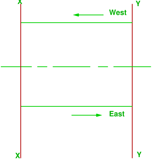
Moving-vehicle method: In this method, the observer moves in the traffic stream and makes
a round trip on a test section. The observer starts at section, drives the car in a particular
direction say eastward to another section, turns the vehicle around drives in the opposite
direction say westward toward the previous section again. Let, the time in minutes it takes
to travel east (from X-X to Y-Y) is ta, the time in minutes it takes to travel west (from Y-Y
to X-X) is tw, the number of vehicles traveling east in the opposite lane while the test car is
traveling west be ma, the number of vehicles that overtake the test car while it is traveling west
be mo, and the number of vehicles that the test car passes while it is traveling west from be mp.
Figure 1: Illustration of moving observer method
The volume (qw) in the westbound direction can then be obtained from the expression and \begin {equation*} qw=\frac {ma+mo-mp}{ta+tw} \end {equation*} the
average travel time in the westbound direction is obtained from \begin {equation*} tw(avg)=tw-\frac {mo-mp}{qw} \end {equation*}
Maximum-car method: In this procedure, the driver is asked to drive as fast as is safely practical
in the traffic stream without ever exceeding the design speed of the facility.
Elevated Observer method: In urban areas, it is sometime possible to station observers in high
buildings or other elevated points from which a considerable length of route may be observed. These
investigator select vehicle at random and record; time, location and causes-of-delay. The drawback is
that it is sometime difficult to secure suitable points for observation throughout the length of the
route to be studied.
License Plate Method: when the amount of turning off and on the route is not great and only
over all speed value are to be secured, the license-plate method of speed study may be satisfactorily
employed. Investigator stationed at control point along the route enters, on a time control basis, the
license-plate numbers of passing vehicles. These are compared from point to point along the route,
and the difference in time values, through use of synchronized watches, is computed. This method
requires careful and time-consuming office work and does not show locations, causes, frequency, or
duration of delay. Four basic methods of collecting and processing license plates normally considered
are:
Manual: collecting license plates via pen and paper or audio tape recorders and manually
entering license plates and arrival times into a computer.
Portable Computer: collecting license plates in the field using portable computers
that automatically provide an arrival time stamp.
Video with Manual Transcription: collecting license plates in the field using video
cameras or camcorders and manually transcribing license plates using human observers.
Video with Character Recognition: collecting license plates in the field using video,
and then automatically transcribing license plates and arrival times into a computer
using computerized license plate character recognition.
Photographic Method: This method is primarily a research tool, it is useful in studies of
interrelationship of several factors such as spacing, speeds, lane usage, acceleration rates, merging
and crossing maneuvers, and delays at intersections. This method is applicable to a short test section
only.
Interview Method: this method may be useful where a large amount of material is needed in a
minimum of time and at little expense for field observation. Usually the employees of a farm or
establishment are asked to record their travel time to and from work on a particular
day.
Highway Capacity Manual 2000 or (Cycle- based method): This method is applicable to all
under saturated signalized intersections. For over-saturated conditions, queue buildup normally
makes the method impractical. The method described here is applicable to situations in
which the average maximum queue per cycle is no more than about 20 to 25 veh/ln.
When queues are long or the demand to capacity ratio is near 1.0, care must be taken to
continue the vehicle-in-queue count past the end of the arrival count period, vehicles that
arrived during the survey period until all of them have exited the intersection.as detailed
below. This requirement is for consistency with the analytic delay equation used in the
chapter text.method does not directly measure delay during deceleration and during a
portion of acceleration, which are very difficult to measure without sophisticated tracking
equipment. However, this method has been shown to yield a reasonable estimate of control
delay.
The method includes an adjustment for errors that may occurred when this type of sampling
technique is used, as well as an acceleration-deceleration delay correction factor Table 1. The
acceleration-deceleration factor is a function of the typical number of vehicles in queue during each
cycle and the normal free-flow speed when vehicles are unimpeded by the signal. Before beginning
the detailed survey, the observers need to make an estimate of the average free-flow speed during the
study period. Free-flow speed is the speed at which vehicles would pass unimpeded through
the intersection if the signal were green for an extended period.be obtained by driving
through the intersection a few times when the signal is green and there is no queue
and recording the speed at a location least affected by signal control. Typically, the
recording location should be upstream about mid-block. Table 2 is a worksheet that
can be used for recording observations and computation of average time-in-queue delay
Sum each column of vehicle-in-queue counts, then sum the column totals for the entire
survey period.
A vehicle recorded as part of a vehicle-in-queue count is in queue, on average, for the time
interval between counts. The average time-in-queue per vehicle arriving during the
survey period is estimated. \begin {equation*} d_{vq}=\left (Is\times \frac {\Sigma V_{iq}}{V_{tot}}\right )0.9 \end {equation*} where, Is = interval between vehicle-in-queue counts
(s), \(\Sigma V_{iq}\) = sum of vehicle-in-queue counts (veh), \(V_{tot}\) = total number of vehicles arriving
during the survey period (veh), and 0.9 = empirical adjustment factor. The 0.9
adjustment factor accounts for the errors that may occur when this type of sampling
technique is used to derive actual delay values, normally resulting in an overestimate of
delay.
Compute the fraction of vehicles stopping and the average number of vehicles stopping per lane
in each signal cycle, as indicated on the worksheet.
Using Table 1, look up a correction factor appropriate to the lane group free-flow speed and the
average number of vehicles stopping per lane in each cycle. This factor adds an adjustment for
deceleration and acceleration delay, which cannot be measured directly with manual
techniques.
Multiply the correction factor by the fraction of vehicles stopping,
and then add this product to the time-in-queue value of Step
2 to obtain the final estimate of control delay per vehicle.
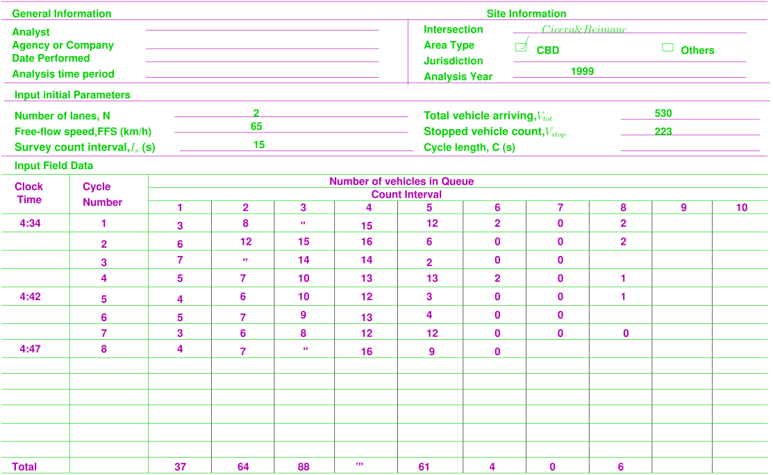
Figure 2: Intersection delay worksheet
6.0.1 Numerical Example
A test was conducted to determine the delay in an intersection. Table 3 presents a sample computation on
direct observation of vehicle-in-queue counts at the intersection. The traffic signal at the intersection
operates with a cycle time of 115 sec. The test was conducted on the 2 lane road over a 15-min period,
which is almost thirteen cycles . Count interval was 15-s. The total number of vehicle is 530 and the total
number of stopped vehicle is 223. Assume the free flow speed to be 65 km/h and the empirical adjustment
factor 0.9
Figure 3: Example of the intersection control delay worksheet
The information assembled as part of this travel time and delay study forms a baseline for future
assessment. This study helps to determine the amount of time required to travel from one
point to another on a given route. Often, information may also be collected on the locations,
durations, and causes of delays. Good indication of the level of service and identifying problem
locations
Exercises
It was observed that the inductive loop was on for 0.39, 0.46, 0.43, 0.47, 0.50, 0.51, 0.48,
0.46, 0.32, 0.44, 0.50, 0.45, 0.44 seconds during one minute interval. If the effective length of
a vehicle is 7 meters, compute the density.
The on and off time (in sec) of a presence type detector are given below. Compute the flow in
veh/hr, occupancy in percentage, density in veh/km, time mean speed and space mean speed in
km/hr. Given that the duration of observation is 60 seconds, the length of the detector is 4 meters
and the length of the vehicle is 5 meters.
\(i\)
\(t_i^{on}\)
\(t_i^{off}\)
1
7.11
7.34
2
16.47
17.13
3
26.10
26.47
4
36.54
37.31
5
43.20
43.56
6
55.00
55.42
References
Highway capacity manual, 2000. chapter-16.
Manual on uniform traffic studies, 2000. Topic No. 750-020-007 Travel Time and Delay Study.
Travel Time Data Collection Handbook. 2019.
F D Hobbs. Traffic Planning and Engineering. Pergamon Press, 1979. 2nd Edition.
W S Hamburger J H Kell. Fundamentals of Traffic Engineering. 1989.
Theodore M Matson, Wilbur S Smith, and Frederick W Hurd. Traffic Engineering. McGraw
Hill Book Company, New York, 1955.
Acknowledgments
I wish to thank several of my students and staff of NPTEL for their contribution in this lecture. I
also appreciate your constructive feedback which may be sent to tvm@civil.iitb.ac.in. Prof.
Tom V. Mathew, Department of Civil engineering, Indian Instiute of Technology Bombay,
India.