Modelling arrival of vehicle at section of road is an important step in traffic flow modelling. It has important application in traffic flow simulation where vehicles are to be generated how vehicles arrive at a section. The vehicle arrival is obviously a random process. This is evident if one observe how vehicles are arriving at a cross section. Some times several vehicles come together, while at other times, they come sparsely. Hence, vehicle arrival at a section need to be characterized statistically. Vehicle arrivals can be modelled in two inter-related ways; namely modelling what is the time interval between the successive arrival of vehicles or modelling how many vehicle arrive in a given interval of time. In the former approach, the random variables the time denoting interval between successive arrival of vehicle can be any positive real values and hence some suitable continuous distribution can be used to model the vehicle arrival. In the later approach, the random variables represent the number of vehicles arrived in a given interval of time and hence takes some integer values. Here in this approach, a discrete distribution can be used to model the process. This chapter presents how some continuous distributions can be used to model the vehicle arrival process.
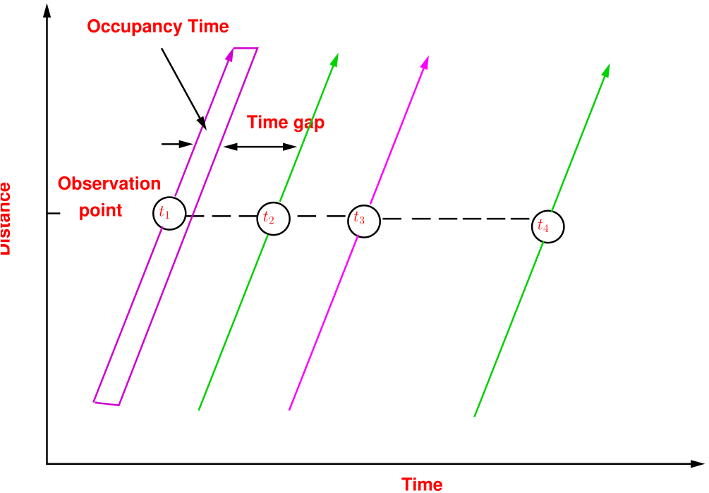
An important parameter to characterize the traffic is to model the inter-arrival time of vehicle at a section on the road. The inter-arrival time or the time headway is not constant due to the stochastic nature of vehicle arrival. A common way of modeling to treat the inter-arrival time or the time headway as a random variable and use some mathematical distributions to model them. The behavior of vehicle arrival is different at different flow condition. It may be possible that different distributions may work better at different flow conditions. Suppose the vehicle arrive at a point at time \(t_1,t_2,\dots \). Then the time difference between two consecutive arrivals is defined as headway. This is shown as a time-distance diagram in figure 1.
In fact the headway consist of two components, the occupancy time which is the duration required for the vehicle to pass the observation point and the time gap between the rear of the lead vehicle and front of the following vehicle. Hence, the headways \(h_1=t_2-t_1,~h_2=t_3-t_2,~\dots \) It may be noted that the headways \(h_1,~h_2,~\dots \) will not be constant, but follows some random distribution. Further, under various traffic states, different distribution may best explain the arrival pattern. A brief discussion of the various traffic states and suitable distributions are discussed next. Generally, traffic state can be divided into three; namely low, medium and high flow conditions. Salient features of each of the flow state is presented below after a brief discussion of the probability distribution.
Low volume flow
High volume flow
Intermediate flow
The low flow traffic can be modeled using the negative exponential distribution. First, some basics of negative exponential distribution is presented. The probability density function \(f(t)\) of any distribution has the following two important properties: First,
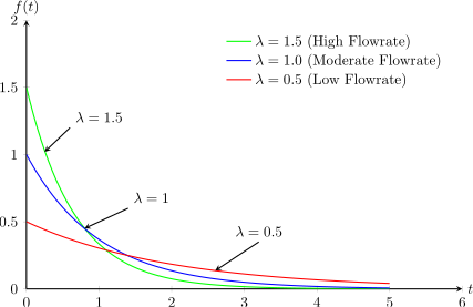
where \(t\) is the random variable. This means that the total probability defined by the probability density function is one. Second: \begin {equation} p[a \le t\le b]=\int _{a}^{b}f(t)~dt \end {equation} This gives an expression for the probability that the random variable \(t\) takes a value with in an interval, which is essentially the area under the probability density function curve. The probability density function of negative exponential distribution is given as: \begin {equation} f(t)=\lambda e^{-\lambda t},~~~t\ge 0 \end {equation} where \(\lambda \) is a parameter that determines the shape of the distribution often called as the shape parameter. The shape of the negative exponential distribution for various values of \(\lambda \) (0.5, 1, 1.5) is shown in figure 2.
The probability that the random variable \(t\) is greater than or equal to zero can be derived as follow,
The probability that the random variable \(t\) is greater than a specific value \(h\) is given as
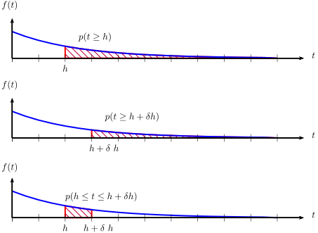
Unlike many other distributions, one of the key advantages of the negative exponential distribution is the existence of a closed form solution to the probability density function as seen above. The probability that the random variable \(t\) lies between an interval is given as:
This is illustrated in figure 3.
The negative exponential distribution is closely related to the Poisson distribution which is a discrete distribution. The probability density function of Poisson distribution is given as: \begin {equation} p(x)=\frac {\lambda ^x~e^{-\lambda }}{x!} \end {equation} where, \(p(x)\) is the probability of \(x\) events (vehicle arrivals) in some time interval (\(t\)), and \(\lambda \) is the expected (mean) arrival rate in that interval. If the mean flow rate is \(q\) vehicles per hour, then \(\lambda =\frac {q}{3600}\) vehicles per second. Now, the probability that zero vehicle arrive in an interval \(t\), denoted as \(p(0)\), will be same as the probability that the headway (inter arrival time) greater than or equal to \(t\). Therefore,
Here, \(\lambda \) is defined as average number of vehicles arriving in time \(t\). If the flow rate is \(q\) vehicles per hour, then, \begin {equation} \lambda =\frac {q\times ~t}{3600}=\frac {t}{\mu } \end {equation} Since mean flow rate is inverse of mean headway, an alternate way of representing the probability density function of negative exponential distribution is given as \begin {equation} f(t)=\frac {1}{\mu }~e^\frac {-t}{\mu } \end {equation} where \(\mu =\frac {1}{\lambda }\) or \(\lambda =\frac {1}{\mu }\). Here, \(\mu \) is the mean headway in seconds which is again the inverse of flow rate. Using equation ?? and equation ?? the probability that headway between any interval and flow rate can be computed. The next example illustrates how a negative exponential distribution can be fitted to an observed headway frequency distribution.
An observation from 2434 samples is given table below. Mean headway and the standard deviation observed is 3.5 and 2.6 seconds respectively. Fit a negative exponential distribution.
| \(h\) | \(h+dh\) | \(p_i^o\) |
| 0.0 | 1.0 | 0.012 |
| 1.0 | 2.0 | 0.178 |
| 2.0 | 3.0 | 0.316 |
| 3.0 | 4.0 | 0.218 |
| 4.0 | 5.0 | 0.108 |
| 5.0 | 6.0 | 0.055 |
| 6.0 | 7.0 | 0.033 |
| 7.0 | 8.0 | 0.022 |
| 8.0 | 9.0 | 0.013 |
| 9.0 | \(>\) | 0.045 |
| Total | 1.00 | |
Solution: The solution is shown in Table 2. The headway range and the observed probability (or proportion) is given in column (2), (3) and (4). The observed frequency for the first interval (0 to 1) can be computed as the product of observed frequency \(p_i\) and the number of observation (N). That is, \(f_i^o = p_i\times N = 0.012\times 2434 = 29.21\) and is shown in column (5). The probability that the headway greater than \(t=0\) is computed as \(p(t\ge 0)=e^{-0}=1\) (refer equation ??) and is given in column (6). These steps are repeated for the second interval, that is \(f_i^o=0.178\times 2434=433.25\), and \(p(t\ge 1)=e^{-1}=0.751\). Now, the probability of headway lies between 0 and 1 for the first interval is given by the probability that headway greater than zero from the first interval minus probability that headway greater than one from second interval. That is \(p_i(0\le t\le 1)=p_i(t>0)-p_i(t> 1)=1.00-0.751=0.249\) and is given in column (7). Now the computed frequency \(f_i^c\) is \(p_i\times N = 0.249\times 2434=604.904\) and is given in column (8). This procedure is repeated for all the subsequent items. It may be noted that probability of headway \(>\) 9.0 is computed by 1-probability of headway less than 9.0 \(= 1-(0.249+0.187+\dots )=0.076.\)
| \(No\) | \(h\) | \(h+dh\) | \(p_i^o\) | \(f_i^o\) | \(p(t>=h)\) | \(p_i^c\) | \(f_i^c\) |
| (1) | (2) | (3) | (4) | (5) | (6) | (7) | (8) |
| 1 | 0.0 | 1.0 | 0.012 | 29.21 | 1.000 | 0.249 | 604.904 |
| 2 | 1.0 | 2.0 | 0.178 | 433.25 | 0.751 | 0.187 | 454.572 |
| 3 | 2.0 | 3.0 | 0.316 | 769.14 | 0.565 | 0.140 | 341.600 |
| 4 | 3.0 | 4.0 | 0.218 | 530.61 | 0.424 | 0.105 | 256.705 |
| 5 | 4.0 | 5.0 | 0.108 | 262.87 | 0.319 | 0.079 | 192.908 |
| 6 | 5.0 | 6.0 | 0.055 | 133.87 | 0.240 | 0.060 | 144.966 |
| 7 | 6.0 | 7.0 | 0.033 | 80.32 | 0.180 | 0.045 | 108.939 |
| 8 | 7.0 | 8.0 | 0.022 | 53.55 | 0.135 | 0.034 | 81.865 |
| 9 | 8.0 | 9.0 | 0.013 | 31.64 | 0.102 | 0.025 | 61.520 |
| 10 | 9.0 | \(>\) | 0.045 | 109.53 | 0.076 | 0.076 | 186.022 |
| Total | 2434 | 1.000 | 2434 | ||||
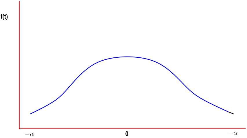
The probability density function of the normal distribution is given by: \begin {equation} f(t)=\frac {1}{\sigma \sqrt {2\pi }} e^{\frac {-(t-\mu )^2}{2\sigma ^2}};-\infty < t <\infty , -\infty < \mu <\infty ,\sigma >0 \end {equation} where \(\mu \) is the mean of the headway and \(\sigma \) is the standard deviation of the headways. The shape of the probability density function is shown in figure 4.
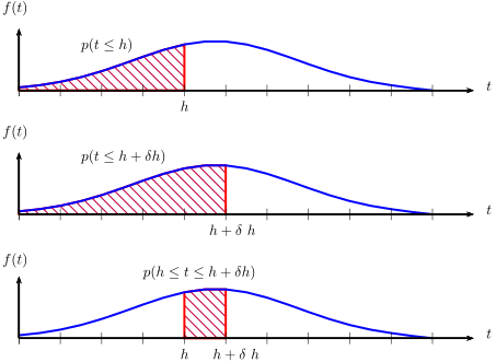
The probability that the time headway (t) less than a given time headway (h) is given by
and the value of this is shown as the area under the curve in figure 5 (a) and the probability of time headway (t) less than a given time headway (\(h+\delta h\)) is given by
This is shown as the area under the curve in figure 5 (b). Hence, the probability that the time headway lies in an interval, say \(h\) and \(h+\delta h\) is given by
This is illustrated as the area under the curve in figure 5 (c).
Although the probability for headway for an interval can be computed easily using equation ??, there is no closed form solution to the equation ??. Even though it is possible to solve the above equation by numerical integration, the computations are time consuming for regular applications. One way to overcome this difficulty is to use the standard normal distribution table which gives the solution to the equation ?? for a standard normal distribution. A standard normal distribution is normal distribution of a random variable whose mean is zero and standard deviation is one. The probability for any random variable, having a mean (\(\mu \)) and standard deviation (\(\sigma \)) can be computed by normalizing that random variable with respect to its mean and standard deviation and then use the standard normal distribution table. This is based on the concept of normalizing any normal distribution based on the assumption that if t follows normal distribution with mean \(\mu \) and standard deviation \(\sigma \), then \((t-\mu )/\sigma \) follows a standard normal distribution having zero mean and unit standard deviation. The normalization steps shown below.
The first and second term in this equation be obtained from standard normal distribution table. The following example illustrates this procedure.
If the mean and standard deviation of certain observed set of headways is 2.25 and 0.875 respectively, then compute the probability that the headway lies in an interval of 1.5 to 2.0 seconds.
Solution: The probability that headway lies between 1.5 and 2.0 can be obtained using equation ??, given that \(\mu =2.25\) and \(\sigma =0.85\) as:
Note that the \(p(t\le -0.29)\) and \(p(t\le -0.80)\) are obtained from the standard normal distribution tables. Since the normal distribution is defined from \(-\alpha \) to \(+\alpha \) unlike an exponential distribution which is defined only for positive number, it is possible that normal distribution may generate negative headways. A practical way of avoiding this is to shift the distribution by some value so that it will mostly generate realistic headways. The concept is illustrated in figure 6.
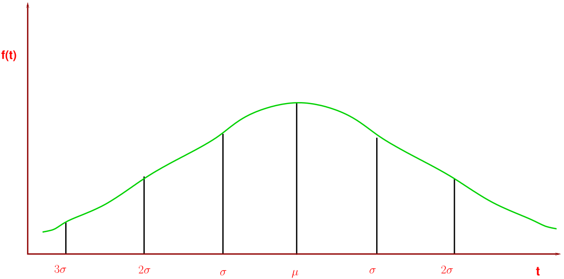
Suppose \(\alpha \) is the minimum possible headway and if we set \(\alpha = \mu -\sigma \) than about 60% of headway will be greater than \(\alpha \). Alternatively, if we set \(\alpha =\mu -2\sigma \), than about 90% of the headway will be greater than \(\alpha \). Further, if we set \(\alpha =\mu -3\sigma \), than about 99% of the headway will be greater than \(\alpha \). To generalize,
where n is 1, 2, 3, etc and higher the value of \(n\), then is better the precision. From this equation, we can compute the value of \(\sigma \) to be used in normal distribution calculation when the random variable cannot be negative as:
Given that observed mean headway is 3.5 seconds and standard distribution is 2.6 seconds, then compute the probability that the headway lies between 0 and 0.5. Assume that the minimum expected headway is 0.5 seconds.
Solution: First, compute the standard deviation to be used in calculation using equation ??, given that \(\mu =3.5\), \(\sigma =2.6\), and \(\alpha =0.5\). Then: \begin {equation} \sigma =\frac {\mu -\alpha }{2}=\frac {3.5-0.5}{2}=1.5 \end {equation} Second, compute the probability that headway less than zero.
The value 0.01 is obtained from standard normal distribution table. Similarly, compute the probability that headway less than 0.5 as
The value 0.23 is obtained from the standard normal distribution table. Hence, the probability that headway lies between 0 and 0.5 is obtained using equation ?? as \(p(0\le t\le 0.5)\)=\( 0.023-0.010 = 0.023\).
An observation from 2434 samples is given table below. Mean headway observed was 3.5 seconds and the standard deviation observed was 2.6 seconds. Fit a normal distribution, if we assume minimum expected headway is 0.5.
| \(h\) | \(h+dh\) | \(p_i^o\) |
| 0.0 | 1.0 | 0.012 |
| 1.0 | 2.0 | 0.178 |
| 2.0 | 3.0 | 0.316 |
| 3.0 | 4.0 | 0.218 |
| 4.0 | 5.0 | 0.108 |
| 5.0 | 6.0 | 0.055 |
| 6.0 | 7.0 | 0.033 |
| 7.0 | 8.0 | 0.022 |
| 8.0 | 9.0 | 0.013 |
| 9.0 | \(>\) | 0.045 |
| Total | 1.00 | |
Solutions The given headway range and the observed probability is given in column (2), (3) and (4). The observed frequency for the first interval (0 to 1) can be computed as the product of observed frequency \(p_i\) and the number of observation (N) i.e. \(p_i^o = p_i\times N = 0.012\times 2434 = 29.21\) as shown in column (5). Compute the standard deviation to be used in calculation, given that \(\mu =3.5\), \(\sigma =2.6\), and \(\alpha =0.5\) as:
Second, compute the probability that headway less than zero.
The value 0.01 is obtained for standard normal distribution table is shown in column (6). Similarly, compute the probability that headway less than 1.0 as:
The value 0.048 is obtained from the standard normal distribution table is shown in column (6). Hence, the probability that headway between 0 and 1 is obtained using equation ?? as \(p(0\le t\le 1)\)=\( 0.048-0.010 = 0.038\) and is shown in column (7). Now the computed frequency \(F_i^c\) is \(p(t<h<t+1)\times N = 0.038\times 2434=92.431\) and is given in column (8). This procedure is repeated for all the subsequent items. It may be noted that probability of headway \(>\) 9.0 is computed by one minus probability of headway less than 9.0 \(=1-(0.038+0.111+\dots )=0.010.\)
| \(No\) | \(h\) | \(h+\delta ~h\) | \(p_i^o\) | \(f_i^o=p_i^o\times N\) | \(p(t\leq h)\) | \(p(t<h<t+\delta ~h)\) | \(f_i^c=p_i^c\times N\) |
| (1) | (2) | (3) | (4) | (5) | (6) | (7) | (8) |
| 1 | 0.0 | 1.0 | 0.012 | 29.21 | 0.010 | 0.038 | 92.431 |
| 2 | 1.0 | 2.0 | 0.178 | 433.25 | 0.048 | 0.111 | 269.845 |
| 3 | 2.0 | 3.0 | 0.316 | 769.14 | 0.159 | 0.211 | 513.053 |
| 4 | 3.0 | 4.0 | 0.218 | 530.61 | 0.369 | 0.261 | 635.560 |
| 5 | 4.0 | 5.0 | 0.108 | 262.87 | 0.631 | 0.211 | 513.053 |
| 6 | 5.0 | 6.0 | 0.055 | 133.87 | 0.841 | 0.111 | 269.845 |
| 7 | 6.0 | 7.0 | 0.033 | 80.32 | 0.952 | 0.038 | 92.431 |
| 8 | 7.0 | 8.0 | 0.022 | 53.55 | 0.990 | 0.008 | 20.605 |
| 9 | 8.0 | 9.0 | 0.013 | 31.64 | 0.999 | 0.001 | 2.987 |
| 10 | 9.0 | \(>\) | 0.045 | 109.53 | 1.000 | 0.010 | 24.190 |
| Total | 2434 | ||||||
As noted earlier, the intermediate flow is more complex since certain vehicles will have interaction with the other vehicles and certain may not. Here, Pearson Type III distribution can be used for modelling intermediate flow. The probability density function for the Pearson Type III distribution is given as
where \(\lambda \) is a parameter which is a function of \(\mu \), \(K\) and \(\alpha \), and determine the shape of the distribution. The term \(\mu \) is the mean of the observed headways, K is a user specified parameter greater than 0 and is called as a shift parameter. The \(\Gamma ()\) is the gamma function and given as
It may also be noted that Pearson Type III is a general case of Gamma, Erlang and Negative Exponential distribution as shown in below:
The expression for the probability that the random headway (t) is greater than a given headway (h), \(p(t\ge h)\), is given as:
and similarly \(p(t > h+\delta h)\) is given as:
and hence, the probability that the headway between \(h\) and \(h+\delta h\) is given as
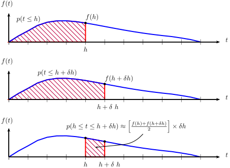
It may be noted that closed form solution to equation ?? and equation ?? is not available. Numerical integration is also difficult due to computational requirement. Using table as in the case of Normal Distribution is difficult, since the table will be different for each \(K\). A common way of solving this is by using the numerical approximation to equation ??. The solution to equation ?? is essentially the area under the curve defined by the probability density function between \(h\) and \(h+\delta h\). If we assume that line joining \(f(h)\) and \(f(h+\delta h)\) is linear, which is a reasonable assumption if \(\delta h\) is small, than the are under the curve can be found out by the following approximate expression:
This concept is illustrated in figure 7
Step wise procedure to fit a Pearson Type III distribution
Compute the shape factor using the mean (\(\mu \)) the standard deviation (\(\sigma \)) and the minimum expected headway (\(\alpha \))
Compute the term flow rate (\(\lambda \)) as
Note that if \(K=1\) and \(\alpha =0\), then \(\lambda =\frac {1}{\mu }\) which is the flow rate.
Compute gamma function value for \(K\) as: \begin {equation} \begin {array}{llll} \Gamma (K) &= (K-1)!&\mathrm {if}~K\in I&(\mathrm {Integer})\\ &=(K-1)~\Gamma (K-1)&\mathrm {if}~K\in R&(\mathrm {Real}) \end {array} \end {equation} Although the closed form solution of \(\Gamma (K)\) is available, it is difficult to compute. Hence, it can be obtained from gamma table. For, example:
Note that the value of \(\Gamma (1.785)\) is obtained from gamma table for \(\Gamma (x)\) which is given for \(1\le x\le 2\).
The Gamma function is defined as: \begin {equation} \Gamma (x)=\int _{0}^{\infty }e^x~x^{n-1}~dx \end {equation} The Gamma function can be evaluated by the following approximate expression also: \begin {equation} \Gamma (x)=x^x~e^{-x}~\sqrt \frac {2~\pi }{x} \left (1+\frac {1}{12~x}+\frac {1}{288x^2}+\dots \right ) \end {equation}
An observation from 2434 samples is given table below. Mean headway observed was 3.5 seconds and the standard deviation 2.6 seconds. Fit a Person Type III Distribution.
| \(h\) | \(h+dh\) | \(p_i^o\) |
| 0.0 | 1.0 | 0.012 |
| 1.0 | 2.0 | 0.178 |
| 2.0 | 3.0 | 0.316 |
| 3.0 | 4.0 | 0.218 |
| 4.0 | 5.0 | 0.108 |
| 5.0 | 6.0 | 0.055 |
| 6.0 | 7.0 | 0.033 |
| 7.0 | 8.0 | 0.022 |
| 8.0 | 9.0 | 0.013 |
| 9.0 | \(>\) | 0.045 |
| Total | 1.00 | |
| \(No\) | \(h\) | \(h+\delta ~h\) | \(p_i^o\) | \(f_i^o\) | \(f(t)\) | \(p_i^c\) | \(f_i^c\) |
| (1) | (2) | (3) | (4) | (5) | (6) | (7) | (8) |
| 1 | 0 | 1 | 0.012 | 29.2 | 0.000 | 0.132 | 321.2 |
| 2 | 1 | 2 | 0.178 | 433.3 | 0.264 | 0.238 | 580.1 |
| 3 | 2 | 3 | 0.316 | 769.1 | 0.213 | 0.185 | 449.5 |
| 4 | 3 | 4 | 0.218 | 530.6 | 0.157 | 0.134 | 327.3 |
| 5 | 4 | 5 | 0.108 | 262.9 | 0.112 | 0.096 | 233.4 |
| 6 | 5 | 6 | 0.055 | 133.9 | 0.079 | 0.068 | 164.6 |
| 7 | 6 | 7 | 0.033 | 80.3 | 0.056 | 0.047 | 115.3 |
| 8 | 7 | 8 | 0.022 | 53.6 | 0.039 | 0.033 | 80.4 |
| 9 | 8 | 9 | 0.013 | 31.6 | 0.027 | 0.023 | 55.9 |
| 10 | \(>\)9 | 0.045 | 109.5 | 0.019 | 0.044 | 106.4 | |
| Total | 1.0 | 2434 | 1.0 | 2434 | |||
Solutions Given that mean headway (\(\mu \)) is 3.5 and the standard deviation (\(\sigma \)) is 2.6. Assuming the expected minimum headway (\(\alpha \)) is 0.5, \(K\) can be computed as
and flow rate term \(\lambda \) as
Now, since \(K=1.15\) which is between 1 and 2, \(\Gamma (K)\) can be obtained directly from the gamma table as \(\Gamma (K)=0.93304\). Here, the probability density function for this example can be expressed as
The given headway range and the observed probability is given in column (2), (3) and (4). The observed frequency (\(f_i^o\)) for the first interval (0 to 1) can be computed as the product of observed proportion \(p_i^o\) and the number of observations (\(N\)). That is, \(f_i^o = p_i^o\times N = 0.012\times 2434 = 29.21\) as shown in column (5). The probability density function value for the lower limit of the first interval (h=0) is shown in column (6) and computed as:
Note that since \(t-\alpha ~(0-0.5)\) is negative and \(K-1~(1.15-1)\) is a fraction, the above expression cannot be evaluated and hence approximated to zero (corresponding to t=0.5). Similarly, the probability density function value for the lower limit of the second interval (h=1) is shown in column 6 and computed as:
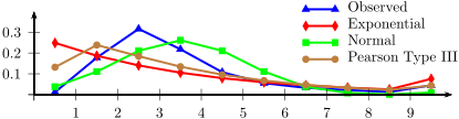
Now, for the first interval, the probability for headway between 0 and 1 is computed by equation ?? as \(p_i^c(0\le t\le 1)=\left (\frac {f(0)+(f(1)}{2}\right )\times (1-0)=(0+0.0264)/2\times ~1=0.132\) and is given in column (7). Now the computed frequency \(f_i^c\) is \(p_i^c\times N = 0.132\times 2434=321.1\) and is given in column (8). This procedure is repeated in all the subsequent rows. It may be noted that probability of headway greater than 9 is computed by subtracting the probability of headway less than 9 from 1; i.e., \(p(t>9)=1-p(t\le 9)=1-(0.132+0.238+\dots )=0.044.\) The comparison of the three distribution for the above data is plotted in Figure 8. It can be noted that none of the distributions exactly replicated the observed distribution. Further, visual observation may not help is judge which is better. This require some objective measure for comparing distribution. One such comparison is using chi-square, which will be covered next chapter.
This chapter covers how the vehicle arrival can be modelled using various distributions. The negative exponential distribution is used when the traffic is low and is most simplest of the distributions in terms of computation effort. The normal distribution on the other hand is used for highly congested traffic and its evaluation require standard normal distribution tables. The Pearson Type III distribution is a most general kind of distribution and can be used intermediate or normal traffic conditions.
(a) Derive the relationship between time mean speed and space mean speed. (b) Write the probability density function for normal distribution and Parson type III distribution and its special cases with various notations used.
An observation of headways for 800 samples is given below. Mean headway and standard deviation observed are 2.76 and 1.79. Fit Pearson type III distribution if the shift parameter is 0.5.
| t | \(t+\delta t\) | Observed Proportion |
| 0.0 | 1.0 | 191 |
| 1.0 | 2.0 | 131 |
| 2.0 | 3.0 | 170 |
| 3.0 | 4.0 | 98 |
| 4.0 | 5.0 | 82 |
| 5.0 | 6.0 | 81 |
| 6.0 | 7.0 | 44 |
| \(>\) 7.0 | 2 | |
An observer counts 300 vehicles in an hour at a location. Assuming that the vehicle arrival follows Poisson distribution: (i) estimate the probability of a pedestrian getting a gap of at least 5 seconds; and (ii) estimate how many vehicles will be generated in two minutes (Assume 20 second interval and use the following random numbers: 0.60, 0.42, 0.54, 0.48, 0.69, 0.42)
Solution (i) Option 1: Mean arrival rate per 5 second \(\lambda \) is 300/3600*5=5/12. The probability that he will get a gap of 5 second is same that there is no vehile arrival in 5 second interval. So, the required probability si \(p(x=0)=e^{-\lambda }=e^{-5/12}\)=0.659. Option 2: Poisson vehicle arrival means headways follows negative exponential. The mean headway \(\mu \)=300/3600=1/12. The probability that he will get a gap of at least 5 seconds is \(p(t>5)=e^{-h/\mu }=e^{-5/12}\)=0.659.
(ii) Flow rate \(\lambda \) for 20 second interval is 300/3600*20=5/3. Using this compute probability for 0, 1, 2, etc. vehicle arrivals and their cumulative as shown in table below:
| \(x\) | \(p(x)=\frac {\lambda ^x~e^{-\lambda }}{x!}\) | \(\sum p(x)\) |
| 0 | 0.19 | 0.19 |
| 1 | 0.31 | 0.50 |
| 2 | 0.26 | 0.76 |
| 3 | 0.14 | 0.90 |
| No | Random No | Vehicles |
| 1 | 0.60 | 2 |
| 2 | 0.42 | 1 |
| 3 | 0.54 | 2 |
| 4 | 0.48 | 1 |
| 5 | 0.69 | 2 |
| 6 | 0.42 | 1 |
Using the following random numbers generate vehicle arrival for a period of 20 sec. Assume headways to follow exponential distribution with mean time headway 6 sec. \(\left [0.59, 0.45, 0.26, 0.70,0.14, 0.28 \right ]\)
similarly, other headways are as follows.
| Vehicle no. | RN | Headway | Cu.Headway |
| 1 | 0.59 | 5.43 | 5.43 |
| 2 | 0.45 | 3.57 | 9 |
| 3 | 0.26 | 1.8 | 10.8 |
| 4 | 0.70 | 7.2 | 18 |
| 5 | 0.14 | 2.0 | 20 |
At a particular section on a highway the following headways are observed: 0.04, 1.37, 1.98, 5.09, 3.00, 2.32, 2.54, 1.37, 0.94, 1.79, 1.10, 6.24, 4.82, 2.77, 4.82, 6.44. Fit an exponential distribution and compare the observed and estimated mean. [Assume headway ranges as 0-2, 2-4, 4-6, and 6-8]
| Observed | Negative Exponential
| |||||
| Interval | Freq (\(F_{obs}\)) | Prob (p) | \(p(h>t)\) | p(l-h) | \(F_{est}\) | \(h_{est}\) |
| 0-2 | 7 | 0.44 | 1.00 | 0.497 | 7.945 | 7.945 |
| 2-4 | 4 | 0.25 | 0.50 | 0.250 | 4.000 | 11.999 |
| 4-6 | 3 | 0.19 | 0.25 | 0.126 | 2.014 | 10.069 |
| 6-8 | 2 | 0.13 | 0.13 | 0.063 | 1.014 | 7.097 |
| Sum | 16 | 0.06 | mean | 2.319 | ||
A headway survey gave a mean of 3.76 and standard deviation of 1.17. Fit a Pearson type III distribution and find probability that the headway is between 2 and 4 seconds. Assume a shift parameter of 0.5 and an interval of 0.5 for calculations.
Solution: \[ \begin {array}{l} \alpha = 0.5 \\ \\ k = \frac {{\mu - \alpha }}{\sigma } = \frac {{3.76 - 0.5}}{{1.17}} = 2.785 \\ \\ \lambda = \frac {k}{{\mu - \alpha }} = \frac {{2.785}}{{3.76 - 0.5}} = 0.854 \\ \\ \Gamma (2.785) = 1.785*\Gamma (1.785) = 1.655 \\ \\ f(t) = \frac {\lambda }{\Gamma }[\lambda (t - \alpha )]^{k - 1} e^{ - \lambda (t - \alpha )} = \frac {{0.854}}{{1.655}}[0.854(t - 0.5)]^{1.785} e^{ - 0.854(t - 0.5)} \\ \\ \end {array} \] \[ therefore Probability = \frac {{0.5}}{2}[f(2) + f(4) + 2(f(2.5) + f(3.0) + f(3.5))] = 0.447 \]
If the flow rate at a given section of road is 1600 and if we assume the inter arrival time of vehicles follow an exponential distribution, then:
Solution: \[ \begin {array}{l} \lambda = \frac {{1600}}{{3600}} = \frac {4}{9}veh/s \\ \\ x = \frac {9}{4}s/veh \\ \\ f(x) = \lambda e^{ - \lambda x} \\ \\ 1:p(x > 1.8) = 1 - p(x \le 1.8) \\ \\ = e^{ - \frac {4}{9}*1.8} = 0.449 \\ \\ 2:p(1.2 < x < 2.4) = p(x \le 2.4) - p(x \le 1.2) \\ = e^{ - \frac {4}{9}*1.2} - e^{ - \frac {4}{9}*2.4} = 0.242 \\ \\ 3:p(x \le 2.25) = 1 - e^{ - 1} = 0.632 \\ \\ \end {array} \]
An obseravtion from 3424 samples is given table below. Mean headway observed was 3.5 seconds and the standard deviation 2.6 seconds. Fit a negative exponetial distribution.
| \(h\) | \(h+dh\) | \(p_i^{obs}\) |
| 0.0 | 0.5 | 0.012 |
| 0.5 | 1.0 | 0.064 |
| 1.0 | 1.5 | 0.114 |
| 1.5 | 2.0 | 0.159 |
| 2.0 | 2.5 | 0.157 |
| 2.5 | 3.0 | 0.130 |
| 3.0 | 3.5 | 0.088 |
| 3.5 | 4.0 | 0.065 |
| 4.0 | 4.5 | 0.043 |
| 4.5 | 5.0 | 0.033 |
| 5.0 | 5.5 | 0.022 |
| 5.5 | 6.0 | 0.019 |
| 6.0 | 6.5 | 0.014 |
| 6.5 | 7.0 | 0.010 |
| 7.0 | 7.5 | 0.012 |
| 7.5 | 8.0 | 0.008 |
| 8.0 | 8.5 | 0.005 |
| 8.5 | 9.0 | 0.007 |
| 9.0 | 9.5 | 0.005 |
| 9.5 | \(>\) | 0.033 |
| Total | 1.00 | |
Solution: The given headway range and the observed probability is given in column (2), (3) and (4). The observed frequency for the first interval (0 to 0.5) can be computed as the product of observed frequency \(p_i\) and the number of observation (N) i.e. \(p_i^{obs} = p_i\times N = 0.012\times 3424 = 41.1\) as shown in column (5). The probability that the headway greater than \(t=0\) is given by equation ?? that is \(p(t\ge 0)=e^{-0}=1\) and is given in column (6). These steps are repeated for the second interval, that is \(p_i^{obs}=0.064\times 3424=219.14\), and \(p(t\ge 0.5)=e^{-0.5}=0.867\). Now for the first interval, the probability for headway lies between 0 and 0.5 is given by the probability that headway \(>\) 0 from the first interval minus probability that headway \(>\) 0.5 for the second interval, that is \(p_i(0\le t\le 0.5)=p_i(t>0)-p_i(t>0.5)=1.00-0.867=0.133\) and is given in column (7). Now the computed frequency \(F_i^{cal}\) is \(p_i\times N = 0.133\times 3424=455.8\) and is given in column (8). This procedure is repeated for all the subsequent items. It may be noted that probability of headway \(>\) 9.5 is computed by 1-probability of headway less than 9.5 \(= 1-0.133+0.115+\dots =0.066.\)
| slno | h | h+dh | \(p_i^{obs}\) | \(F_i^{obs}\) | \(p(t>=h)\) | \(p_i^{cal}\) | \(F_i^{cal}\) |
| (1) | (2) | (3) | (4) | (5) | (6) | (7) | (8) |
| 1 | 0.0 | 0.5 | 0.012 | 41.1 | 1.000 | 0.133 | 455.8 |
| 2 | 0.5 | 1.0 | 0.064 | 219.1 | 0.867 | 0.115 | 395.1 |
| 3 | 1.0 | 1.5 | 0.114 | 390.3 | 0.751 | 0.100 | 342.5 |
| 4 | 1.5 | 2.0 | 0.159 | 544.4 | 0.651 | 0.087 | 296.9 |
| 5 | 2.0 | 2.5 | 0.157 | 537.6 | 0.565 | 0.075 | 257.4 |
| 6 | 2.5 | 3.0 | 0.130 | 445.1 | 0.490 | 0.065 | 223.1 |
| 7 | 3.0 | 3.5 | 0.088 | 301.3 | 0.424 | 0.056 | 193.4 |
| 8 | 3.5 | 4.0 | 0.065 | 222.6 | 0.368 | 0.049 | 167.7 |
| 9 | 4.0 | 4.5 | 0.043 | 147.2 | 0.319 | 0.042 | 145.4 |
| 10 | 4.5 | 5.0 | 0.033 | 113.0 | 0.276 | 0.037 | 126.0 |
| 11 | 5.0 | 5.5 | 0.022 | 75.3 | 0.240 | 0.032 | 109.2 |
| 12 | 5.5 | 6.0 | 0.019 | 65.1 | 0.208 | 0.028 | 94.7 |
| 13 | 6.0 | 6.5 | 0.014 | 47.9 | 0.180 | 0.024 | 82.1 |
| 14 | 6.5 | 7.0 | 0.010 | 34.2 | 0.156 | 0.021 | 71.2 |
| 15 | 7.0 | 7.5 | 0.012 | 41.1 | 0.135 | 0.018 | 61.7 |
| 16 | 7.5 | 8.0 | 0.008 | 27.4 | 0.117 | 0.016 | 53.5 |
| 17 | 8.0 | 8.5 | 0.005 | 17.1 | 0.102 | 0.014 | 46.4 |
| 18 | 8.5 | 9.0 | 0.007 | 24.0 | 0.088 | 0.012 | 40.2 |
| 19 | 9.0 | 9.5 | 0.005 | 17.1 | 0.076 | 0.010 | 34.8 |
| 20 | 9.5 | \(>\) | 0.033 | 113.0 | 0.066 | 0.066 | 226.8 |
| Total | 1.000 | 3424 | 1.000 | 3424 | |||
An obseravtion from 3424 samples is given table below. Mean headway observed was 3.5 seconds and the standard deviation 2.6 seconds. Fit a normal distrbution, if we assume minimum expected headway is 0.5.
| h | h+dh | \(p_i^{obs}\) |
| 0.0 | 0.5 | 0.012 |
| 0.5 | 1.0 | 0.064 |
| 1.0 | 1.5 | 0.114 |
| 1.5 | 2.0 | 0.159 |
| 2.0 | 2.5 | 0.157 |
| 2.5 | 3.0 | 0.130 |
| 3.0 | 3.5 | 0.088 |
| 3.5 | 4.0 | 0.065 |
| 4.0 | 4.5 | 0.043 |
| 4.5 | 5.0 | 0.033 |
| 5.0 | 5.5 | 0.022 |
| 5.5 | 6.0 | 0.019 |
| 6.0 | 6.5 | 0.014 |
| 6.5 | 7.0 | 0.010 |
| 7.0 | 7.5 | 0.012 |
| 7.5 | 8.0 | 0.008 |
| 8.0 | 8.5 | 0.005 |
| 8.5 | 9.0 | 0.007 |
| 9.0 | 9.5 | 0.005 |
| 9.5 | \(>\) | 0.033 |
| Total | 1.00 | |
Solution: The given headway range and the observed probability is given in column (2), (3) and (4). Compute the standard deviation to be used in calculation,given that \(\mu =3.5\), \(\sigma =2.6\), and \(\alpha =0.5\).:
Second, compute the probability that headway less than zero.
The value 0.01 is obtained for standard normal distribution table is shown in column (6). Simmilarly, compute the probability that headway less than 0.5 as
The value 0.023 is obtained from the standard normal distribution table is shown in column (6). Hence, the probability that headway between 0 and 1 is obtained using equation ?? as \(p(0\le t\le 0.5)\)=\( 0.023-0.010 = 0.013\) as shown in column (7). Now the computed frequency \(F_i^cal\) is \(p(t<h<t+1)\times N = 0.013\times 3424=44.289\) and is given in column (8). This procedure is repeated for all the subsequent items. It may be noted that probability of headway \(>\) 9.5 is computed by 1-probability of headway less than 9.5 \(= 1-0.013+0.025+\dots =0.010.\)
| sl.no | \(h\) | \(h+dh\) | \( pi(obs)\) | \(P=p\times N\) | \(p(h<=t)\) | \(p(t<h<t+0.5)\) | \(P=p\times N\) |
| (1) | (2) | (3) | (4) | (5) | (6) | (7) | (8) |
| 1 | 0.0 | 0.5 | 0.012 | 41.09 | 0.010 | 0.013 | 44.289 |
| 2 | 0.5 | 1.0 | 0.064 | 219.14 | 0.023 | 0.025 | 85.738 |
| 3 | 1.0 | 1.5 | 0.114 | 390.34 | 0.048 | 0.043 | 148.673 |
| 4 | 1.5 | 2.0 | 0.159 | 544.42 | 0.091 | 0.067 | 230.928 |
| 5 | 2.0 | 2.5 | 0.157 | 537.57 | 0.159 | 0.094 | 321.299 |
| 6 | 2.5 | 3.0 | 0.13 | 445.12 | 0.252 | 0.117 | 400.433 |
| 7 | 3.0 | 3.5 | 0.088 | 301.31 | 0.369 | 0.131 | 447.033 |
| 8 | 3.5 | 4.0 | 0.065 | 222.56 | 0.500 | 0.131 | 447.033 |
| 9 | 4.0 | 4.5 | 0.043 | 147.23 | 0.631 | 0.117 | 400.433 |
| 10 | 4.5 | 5.0 | 0.033 | 112.99 | 0.748 | 0.094 | 321.299 |
| 11 | 5.0 | 5.5 | 0.022 | 75.33 | 0.841 | 0.067 | 230.928 |
| 12 | 5.5 | 6.0 | 0.019 | 65.06 | 0.909 | 0.043 | 148.673 |
| 13 | 6.0 | 6.5 | 0.014 | 47.94 | 0.952 | 0.025 | 85.738 |
| 14 | 6.5 | 7.0 | 0.01 | 34.24 | 0.977 | 0.013 | 44.289 |
| 15 | 7.0 | 7.5 | 0.012 | 41.09 | 0.990 | 0.006 | 20.492 |
| 16 | 7.5 | 8.0 | 0.008 | 27.39 | 0.996 | 0.002 | 8.493 |
| 17 | 8.0 | 8.5 | 0.005 | 17.12 | 0.999 | 0.001 | 3.153 |
| 18 | 8.5 | 9.0 | 0.007 | 23.97 | 1.000 | 0.000 | 1.048 |
| 19 | 9.0 | 9.5 | 0.005 | 17.12 | 1.000 | 0.000 | 0.312 |
| 20 | 9.5 | \(>\) | 0.033 | 112.99 | 1.000 | 0.010 | 33.716 |
| Total | 3424 | ||||||
An obseravtion from 3424 samples is given table below. Mean headway observed was 3.5 seconds and the standard deviation 2.6 seconds. Fit a Person Type III Distribution.
| h | h+dh | \(p_iobs\) |
| 0.0 | 0.5 | 0.012 |
| 0.5 | 1.0 | 0.064 |
| 1.0 | 1.5 | 0.114 |
| 1.5 | 2.0 | 0.159 |
| 2.0 | 2.5 | 0.157 |
| 2.5 | 3.0 | 0.130 |
| 3.0 | 3.5 | 0.088 |
| 3.5 | 4.0 | 0.065 |
| 4.0 | 4.5 | 0.043 |
| 4.5 | 5.0 | 0.033 |
| 5.0 | 5.5 | 0.022 |
| 5.5 | 6.0 | 0.019 |
| 6.0 | 6.5 | 0.014 |
| 6.5 | 7.0 | 0.010 |
| 7.0 | 7.5 | 0.012 |
| 7.5 | 8.0 | 0.008 |
| 8.0 | 8.5 | 0.005 |
| 8.5 | 9.0 | 0.007 |
| 9.0 | 9.5 | 0.005 |
| 9.5 | \(>\) | 0.033 |
| Total | 1.00 | |
Solution: Given that mean headway \(\mu =3.5\) and, the standard deviation \(\sigma =2.6\). Assuming the expected minimum headway \(\alpha =0.5\), \(K\) can be computed as
and flow rate term \(\lambda \) as
Now, since \(K=1.15\) which is between 1 and 2, \(\Gamma (K)\) can be obtained directly from the gamma table as \(\Gamma (K)=0.93304\). Here, the probability density function for this example can be expressed as
The given headway range and the observed probability is given in column (2), (3) and (4). The observed frequency for the first interval(0 to 0.5)can be computed as the product of observed frequency \(p_i\) and the number of observation(N) i.e. \(p_i^{obs} = p_i\times N = 0.012\times 3424 = 41.1\) as shown in column (5). The probability that the headway greater than \(t=0\) is given by equation ?? that is \(p(t\ge 0)=e^{-0}=1\) and is given in column (6). These steps are repeated for the second interval,that is \(p_i^{obs}=0.064\times 3424=219.1\), and \(p(t\ge 0.5)=e^{-0.5}=0.867\). Now for the first interval, the probability for headway 0 and 0.5 is given by the probability that headway \(>\) 0 fro the first interval minus probability that headway \(>\) 0.5 for the second interval.that is \(p_i(0\le t\le 0.5)=p_i(t>0)-p_i(t>0.5)=1.00-0.867=0.133\) and is given in column (7). Now the computed frequency \(F_i^cal\) is \(p_i\times N = 0.133\times 3424=455.8\) and is given in column (8). This procedure is repeated for all the subsequent items. It may be noted that probability of headway \(>\) 9.5 is computed by 1-probability of headway less than 9.5 \(= 1-0.133+0.115+\dots =0.066.\)
| sl.no | \(h\) | \(h+dh\) | \(p_i^{obs}\) | \(P=p\times N\) | f(t) | \(p(t<h<t+0.5)\) | \(P=p\times N\) |
| (1) | (2) | (3) | (4) | (5) | (6) | (7) | (8) |
| 1 | 0.0 | 0.5 | 0.012 | 41.09 | 0.000 | 0.00 | |
| 2 | 0.5 | 1.0 | 0.064 | 219.14 | 0.000 | 0.066 | 225.91 |
| 3 | 1.0 | 1.5 | 0.114 | 390.34 | 0.264 | 0.127 | 433.26 |
| 4 | 1.5 | 2.0 | 0.159 | 544.42 | 0.242 | 0.114 | 389.45 |
| 5 | 2.0 | 2.5 | 0.157 | 537.57 | 0.213 | 0.099 | 339.13 |
| 6 | 2.5 | 3.0 | 0.13 | 445.12 | 0.183 | 0.085 | 291.12 |
| 7 | 3.0 | 3.5 | 0.088 | 301.31 | 0.157 | 0.072 | 247.86 |
| 8 | 3.5 | 4.0 | 0.065 | 222.56 | 0.133 | 0.061 | 209.90 |
| 9 | 4.0 | 4.5 | 0.043 | 147.23 | 0.112 | 0.052 | 177.08 |
| 10 | 4.5 | 5.0 | 0.033 | 112.99 | 0.095 | 0.044 | 148.97 |
| 11 | 5.0 | 5.5 | 0.022 | 75.33 | 0.079 | 0.037 | 125.04 |
| 12 | 5.5 | 6.0 | 0.019 | 65.06 | 0.067 | 0.031 | 104.78 |
| 13 | 6.0 | 6.5 | 0.014 | 47.94 | 0.056 | 0.026 | 87.67 |
| 14 | 6.5 | 7.0 | 0.01 | 34.24 | 0.047 | 0.021 | 73.28 |
| 15 | 7.0 | 7.5 | 0.012 | 41.09 | 0.039 | 0.018 | 61.18 |
| 16 | 7.5 | 8.0 | 0.008 | 27.39 | 0.033 | 0.015 | 51.04 |
| 17 | 8.0 | 8.5 | 0.005 | 17.12 | 0.027 | 0.012 | 42.54 |
| 18 | 8.5 | 9.0 | 0.007 | 23.97 | 0.023 | 0.010 | 35.44 |
| 19 | 9.0 | 9.5 | 0.005 | 17.12 | 0.019 | 0.009 | 29.51 |
| 20 | 9.5 | \(>\) | 0.033 | 112.99 | 0.016 | 0.102 | 350.83 |
| total | x | 3424 | |||||
– INSERT –
Given the headways observed from a survey is given below. Fit an exponential distribution and compare the actual and computed mean and standard deviation. 5.15, 1.22, 2.65, 2.35, 0.47, 2.8, 7.67, 4.74, 2.42, 4.87, 5.94, 8.58, 9.74, 0.56, 0.66, 6.72, 7.41, 6.94, 2.42, 5.61
| Observed | Negative Exponential | |||||||||||
| t | h+dh | p (obs) | P=p*N | Ph | (m-h)ˆ2*P | t*(1/m) | p(h¿=t) | N-exp (p) | P=p*N | Ph | (m-h)ˆ2*P | |
| 0.0 | 1.0 | 0.15 | 3.00 | 1.50 | 44.47 | 0.00 | 1.00 | 0.20 | 4.03 | 2.01 | 56.34 | |
| 1.0 | 2.0 | 0.05 | 1.00 | 1.50 | 8.12 | 0.22 | 0.80 | 0.16 | 3.22 | 4.83 | 45.97 | |
| 2.0 | 3.0 | 0.25 | 5.00 | 12.50 | 17.11 | 0.45 | 0.64 | 0.13 | 2.57 | 6.42 | 37.34 | |
| 3.0 | 4.0 | 0 | 0.00 | 0.00 | 0.00 | 0.67 | 0.51 | 0.10 | 2.05 | 7.18 | 30.23 | |
| 4.0 | 5.0 | 0.1 | 2.00 | 9.00 | 0.05 | 0.90 | 0.41 | 0.08 | 1.64 | 7.37 | 24.40 | |
| 5.0 | 6.0 | 0.15 | 3.00 | 16.50 | 3.97 | 1.12 | 0.32 | 0.07 | 1.31 | 7.20 | 19.65 | |
| 6.0 | 7.0 | 0.1 | 2.00 | 13.00 | 9.25 | 1.35 | 0.26 | 0.05 | 1.04 | 6.79 | 15.80 | |
| 7.0 | 8.0 | 0.1 | 2.00 | 15.00 | 19.85 | 1.57 | 0.21 | 0.04 | 0.83 | 6.26 | 12.69 | |
| 8.0 | 9.0 | 0.05 | 1.00 | 8.50 | 17.22 | 1.80 | 0.17 | 0.03 | 0.67 | 5.66 | 10.17 | |
| 9.0 | ¿9.0 | 0.05 | 1.00 | 9.50 | 26.52 | 2.02 | 0.13 | 0.13 | 2.64 | 25.10 | 38.33 | |
| 20 | ||||||||||||
| 1 | 20 | 1 | 20 | |||||||||
| Mean | 4.45 | mean (cal) | 4.35 | Mean (exp) | 3.94 | |||||||
| SD | 2.85 | SD (cal) | 2.71 | SD (exp) | 3.81 | |||||||
(OR)
| Observed | Negative Exponential | |||||||||||
| t | h+dh | p (obs) | P=p*N | Ph | (m-h)ˆ2*P | t*(1/m) | p(h¿=t) | N-exp (p) | P=p*N | Ph | (m-h)ˆ2*P | |
| 0.0 | 0.5 | 0.05 | 1.00 | 0.25 | 9.77 | 0.00 | 1.00 | 0.11 | 2.13 | 0.53 | 16.89 | |
| 0.5 | 1.0 | 0.1 | 2.00 | 1.50 | 13.78 | 0.11 | 0.89 | 0.10 | 1.90 | 1.43 | 15.21 | |
| 1.0 | 1.5 | 0.05 | 1.00 | 1.25 | 4.52 | 0.22 | 0.80 | 0.08 | 1.70 | 2.12 | 13.69 | |
| 1.5 | 2.0 | 0 | 0.00 | 0.00 | 0.00 | 0.34 | 0.71 | 0.08 | 1.52 | 2.66 | 12.31 | |
| 2.0 | 2.5 | 0.15 | 3.00 | 6.75 | 3.80 | 0.45 | 0.64 | 0.07 | 1.36 | 3.05 | 11.07 | |
| 2.5 | 3.0 | 0.1 | 2.00 | 5.50 | 0.78 | 0.56 | 0.57 | 0.06 | 1.21 | 3.33 | 9.94 | |
| 3.0 | 3.5 | 0 | 0.00 | 0.00 | 0.00 | 0.67 | 0.51 | 0.05 | 1.08 | 3.52 | 8.92 | |
| 3.5 | 4.0 | 0 | 0.00 | 0.00 | 0.00 | 0.79 | 0.46 | 0.05 | 0.97 | 3.63 | 8.01 | |
| 4.0 | 4.5 | 0 | 0.00 | 0.00 | 0.00 | 0.90 | 0.41 | 0.04 | 0.87 | 3.68 | 7.18 | |
| 4.5 | ¿4.5 | 0.55 | 11.00 | 52.25 | 20.80 | 1.01 | 0.36 | 0.36 | 7.27 | 34.53 | 47.66 | |
| 20 | ||||||||||||
| 1 | 20 | 1 | 20 | |||||||||
| Mean | 4.45 | mean (cal) | 3.38 | Mean (exp) | 2.92 | |||||||
| SD | 2.85 | SD (cal) | 1.63 | SD (exp) | 2.75 | |||||||
I wish to thank several of my students and staff of NPTEL for their contribution in this lecture. I also appreciate your constructive feedback which may be sent to tvm@civil.iitb.ac.in. Prof. Tom V. Mathew, Department of Civil engineering, Indian Instiute of Technology Bombay, India.