Vehicle Arrival Models : Count

Lecture Notes in Transportation Systems Engineering

1 Introduction
2 Poisson Distribution
2.0.1 Numerical Example
3 Random variates following Poisson distribution
3.0.1 Numerical Example
4 Random variates following Exponential distribution
4.0.1 Numerical Example
5 Evaluation of the mathematical distribution
5.1 Mean and Standard deviation
5.2 Chi-square test
5.2.1 Numerical Example
6 Conclusion
Exercises

1 Introduction

As already noted in the previous chapter that vehicle arrivals can be modelled in two inter-related ways; namely modelling how many vehicle arrive in a given interval of time, or modelling what is the time interval between the successive arrival of vehicles. Having discussed in detail the former approach in the previous chapter, the first part of this chapter discuss how a discrete distribution can be used to model the vehicle arrival. Traditionally, Poisson distribution is used to model the random process, the number of vehicles arriving a given time period. The second part will discuss methodologies to generate random vehicle arrivals, be it the generation of random headways or random number of vehicles in a given duration. The third part will elaborate various ways of evaluating the performance of a distribution.

2 Poisson Distribution

Suppose, if we plot the arrival of vehicles at a section as dot in a time axis, it may look like Figure 1.

Figure 1: Illustration of vehicle arrival modeling

Let \(h_1\), \(h_2\), ... etc indicate the headways, then as mentioned earlier, they take some real values. Hence, these headways or inter arrival time can be modelled using some continuous distribution. Also, let \(t_1\), \(t_2\), \(t_3\) and \(t_4\) are four equal time intervals, then the number of vehicles arrived in each of these interval is an integer value. For example, in Fig. 1, 3, 2, 3 and 1 vehicles arrived in time interval \(t_1\), \(t_2\), \(t_3\) and \(t_4\) respectively. Any discrete distribution that best fit the observed number of vehicle arrival in a given time interval can be used. Similarly, any continuous distribution that best fit the observed headways (or inter-arrival time) can be used in modelling. However, since these process are inter-related, the distributions that describe these relations should also be inter-related for better explanation of the phenomenon. Interestingly, there exist distributions that meet the above requirements. First, we will see the distribution to model the number of vehicles arrived in a given duration of time. Poisson distribution is commonly used to describe such a random process. The probability density function of the Poisson distribution is given as: \begin {equation} p(x)= \frac {\mu ^x e^{-\mu }}{x!} \end {equation} where \(p(x)\) is the probability for \(x\) events will occur in the time interval, and \(\mu \) is the expected rate of occurrence of that event in that interval. Some special cases of this distribution is given below.

\begin {eqnarray*} p(0) &=& e^{-\mu } \\ p(1) &=& \frac {\mu e^{-\mu }}{1} = \mu ~p(0) \\ p(2) &=& \frac {\mu ^2 e^{-\mu }}{2!} = \frac {\mu }{2}~p(1) \\ \therefore p(n) &=& \frac {\mu }{n}~p(n-1). \end {eqnarray*}

Since the events are discrete, the probability that certain number of vehicles (\(n\)) arriving in an interval can be computed as:

\begin {eqnarray*} p(x\le n)&=&\sum _{i=0}^{n} p(i),~i\in ~I. \end {eqnarray*}

Similarly, the probability that the number of vehicles arriving in the interval is exactly in a range (between \(a\) and \(b\), both inclusive and \(a<b\)) is given as:

\begin {eqnarray*} p(a\le x\le b)&=&\sum _{i=a}^{b} p(i),~i\in ~I. \end {eqnarray*}

2.0.1 Numerical Example

The hourly flow rate in a road section is 120 vph. Use Poisson distribution to model this vehicle arrival.

Solution: The flow rate is given as (\(\mu \)) = 120 vph = \(\frac {120}{60}\)= 2 vehicle per minute. Hence, the probability of zero vehicles arriving in one minute \(p(0)\) can be computed as follows:

\begin {eqnarray*} p(0)&=&\frac {\mu ^x e^{-\mu }}{x!} = \frac {2^0.e^{-2}}{0!} = 0.135. \end {eqnarray*}

Similarly, the probability of one vehicles arriving in one minute \(p(1)\) is given by,

\begin {eqnarray*} p(1) &=& \frac {\mu ^x e^{-\mu }}{x!} = \frac {2.e^{-2}}{1!} = 0.271. \end {eqnarray*}

Now, the probability that number of vehicles arriving is less than or equal to zero is given as

\begin {eqnarray*} p(x\leq 0)~=~p(0)~=~0.135. \end {eqnarray*}

Similarly, probability that the number of vehicles arriving is less than or equal to 1 is given as:

\begin {eqnarray*} p(x\leq 1)~=~p(0)~+~p(1)~=~0.135~+~0.275~=~0.406. \end {eqnarray*}

Again, the probability that the number of vehicles arriving is between 2 to 4 is given as:

\begin {eqnarray*} p(2\leq x\leq 4)&=&p(2)+p(3)+p(4),\\ &=&.271+.18+.09~=~0.54. \end {eqnarray*}

Now, if the \(p(0)~=~0.135\), then the number of intervals in an hour where there is no vehicle arriving is

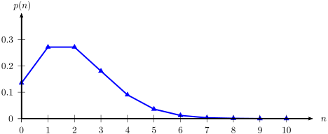
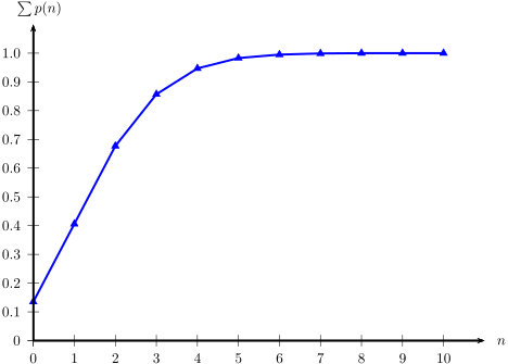
\begin {eqnarray*} F(x)~=~p(0)~\times ~60~=~0.135~\times ~60~=~8.12. \end {eqnarray*}

The above calculations can be repeated for all the cases as tabulated in Table 1.

Table 1: Probability values of vehicle arrivals computed using Poisson distribution


\(n\)	\(p(n)\)	\(p(x\leq n)\)	\(F(n)\)

0	0.135	0.135	8.120

1	0.271	0.406	16.240

2	0.271	0.677	16.240

3	0.180	0.857	10.827

4	0.090	0.947	5.413

5	0.036	0.983	2.165

6	0.012	0.995	0.722

7	0.003	0.999	0.206

8	0.001	1.000	0.052

9	0.000	1.000	0.011

10	0.000	1.000	0.011

The shape of this distribution can be seen from Figure 2 and the corresponding cumulative distribution is shown in Figure 3.

Figure 2: Probability values of vehicle arrivals computed using Poisson distribution

Figure 3: Cumulative probability values of vehicle arrivals computed using Poisson distribution

3 Random variates following Poisson distribution

For simulation purposes, it may be required to generate number of vehicles arrived in a given interval so that it follows typical vehicle arrival. This is the reverse of computing the probabilities as seen above. The following steps give the procedure:

Input: mean arrival rate \(\mu \) in an interval \(t\)
Compute \(p(x=n)\) and \(p(x\leq n)\)
Generate a random number \(X\) such that \(0\leq X\leq 1\)
Find \(n\) such that \(p(x\leq n-1) \le X\) and \(p(x\leq n) \ge X\)
Set \(n_i=n\), where \(n_i\) is the number of vehicles arrived in \(i^{th}\) interval.

The steps 3 to 5 can be repeated for required number of intervals.

3.0.1 Numerical Example

Generate vehicles for ten minutes if the flow rate is 120 vph.

Solution The first two steps of this problem is same as the example problem solved earlier and the resulted from the table is used. For the first interval, the random number (\(X\)) generated is 0.201 which is greater than \(p(0)\) but less than \(p(1)\). Hence, the number of vehicles generated in this interval is one (\(n_i=1\)). Similarly, for the subsequent intervals. It can also be computed that at the end of 10th interval (one minute), total 23 vehicle are generated. Note: This amounts to 2.3 vehicles per minute which is higher than given flow rate. However, this discrepancy is because of the small number of intervals conducted. If this is continued for one hour, then this average will be about 1.78 and if continued for then this average will be close to 2.02.

Table 2: Vehicles generated using Poisson distribution


No	X	n

1	0.201	1

2	0.714	3

3	0.565	2

4	0.257	1

5	0.228	1

6	0.926	4

7	0.634	2

8	0.959	5

9	0.188	1

10	0.832	3

	Total	23

4 Random variates following Exponential distribution

One can generate random variate following negative exponential distribution rather simply due to availability of closed form solutions. The method for generating exponential variates is based on inverse transform sampling:

\begin {eqnarray*} t&=&f^{-1}(X) \end {eqnarray*}

has an exponential distribution, where \(f^{-1}\), called as quantile function, is defined as

\begin {eqnarray*} f^{-1}(X)&=&\frac {\log (1-X)}{\lambda }. \end {eqnarray*}

Note that if \(X\) is uniform, then \(1-X\) is also uniform and \(\lambda =1/\mu \). Hence, one can generate exponential variates as follows:

\begin {eqnarray*} t&=&-\mu \times \log (X) \end {eqnarray*}

where, \(X\) is a random number between 0 and 1, \(\mu \) is the mean headway, and the resultant headways generated (\(t\)) will follow exponential distribution.

4.0.1 Numerical Example

Simulate the headways for 10 vehicles if the flow rate is 120 vph.

Solution Since the given flow rate is 120 vph, then the mean headway (\(\mu \)) is 30 seconds. Generate a random number between 0 and 1 and let this be 0.62. Hence, by the above equation, \(t=30\times (-\log (0.62))=14.57\). Similarly, headways can be generated. The table below given the generation of 15 vehicles and it takes little over 10 minutes. In other words, the table below gives the vehicles generated for 10 minutes. Note: The mean headway obtained from this 15 headways is about 43 seconds; much higher than the given value of 30 seconds. Of, course this is due to the lower sample size. For example, if the generation is continued to 100 vehicles, then the mean would be about 35 seconds, and if continued till 1000 vehicles, then the mean would be about 30.8 seconds.

Table 3: Headways generated using Exponential distribution


No	\(X\)	\(t\)	\(\sum ~t\)

1	0.62	14.57	14.57

2	0.17	53.70	68.27

3	0.27	39.14	107.41

4	0.01	157.36	264.77

5	0.26	40.01	304.78

6	0.47	22.72	327.5

7	0.96	1.38	328.88

8	0.24	42.76	371.64

9	0.59	15.94	387.58

10	0.45	24.05	411.63

11	0.26	40.82	452.45

12	0.11	67.39	519.84

13	0.10	69.33	589.17

14	0.73	9.63	598.8

15	0.31	34.74	633.54

5 Evaluation of the mathematical distribution

The mathematical distribution such as negative exponential distribution, normal distribution, etc needs to be evaluated to see how best these distributions fits the observed data. It can be evaluated by comparing some aggregate statistics as discussed below.

5.1 Mean and Standard deviation

One of the easiest ways to compute the mean and standard deviation of the observed data and compare with mean and standard deviation obtained from the computed frequencies. If \(p_i^c\) is the computed probability of the headway is the \(i^{th}\) interval, and \(N\) is the total number of observations, then the computed frequency of the \(i^{th}\) interval is given as:

\begin {eqnarray*} f_i^c &=& p_i^c\times N. \end {eqnarray*}

Then the mean of the computed frequencies (\(\mu ^c\)) is obtained as

\begin {eqnarray*} \mu ^c &=& \frac {\Sigma f_i^c\times (\frac {2h_i+\delta h}{2})}{N}, \end {eqnarray*}

where \(h_i\) is the lower limit of the \(i^{th}\) interval, and \(\delta h\) is the interval range. The standard deviation \(\sigma ^c\) can be obtained by

\begin {eqnarray*} \sigma ^c &=& \frac {\Sigma (h_i^m - \mu ^c)^2 f_i^c}{N}. \end {eqnarray*}

If the distribution fit closely, then the mean and the standard deviation of the observed and fitted data will match. However, it is possible, that two sample can have similar mean and standard deviation, but, may differ widely in the individual interval. Hence, this can be considered as a quick test for the comparison purposes. For better comparison, Chi-square test which gives a better description of the suitability of the distribution may be used.

5.2 Chi-square test

The Chi-square value (\(X^2\)) can be computed using the following formula:

\begin {eqnarray*} X^2_C &=& \sum _{i=1}^{n}\frac {(f_i^o-f_i^c)^2}{f_i^c} \end {eqnarray*}

where \(f_i^o\) is the observed frequency, \(f_i^c\) is the computed (theoretical) frequency of the \(i^{th}\) interval, and \(n\) is the number of intervals. Obviously, a \(X^2\) value close to zero implies a good fit of the data, while, high \(X^2\) value indicate poor fit. For an objective comparison Chi-square tables are used. A chi-square table gives \(X^2\) values for various degree of freedom. The degree of freedom (DOF) is given as

\begin {eqnarray*} DOF &=& n-1-p \end {eqnarray*}

where n is the number of intervals, and p is the number of parameter defining the distribution. Since negative exponential distribution is defined by mean headway alone, the value of p is one, where as Pearson and Normal distribution has the value of p as two, since they are defined by \(\mu \) and \(\sigma \). Chi-square value is obtained from various significant levels. For example, a significance level of 0.05 implies that the likelihood that the observed frequencies following the theoretical distribution is is 5%. In other words, one could say with 95% confidence that the observed data follows the theoretical distribution under testing.

5.2.1 Numerical Example

Compute the \(X^2\) statistic of the following distribution, where \(N=2434\).

Table 4: \(\chi ^2\)distribution


\(h\)	\(h+dh\)	\(p_i^o\)	\(p_i^c\)

0.0	1	0.012	0.249

1.0	2	0.178	0.187

2.0	3	0.316	0.140

3.0	4	0.218	0.105

4.0	5	0.108	0.079

5.0	6	0.055	0.060

6.0	7	0.033	0.045

7.0	8	0.022	0.034

8.0	9	0.013	0.025

9.0	\(>\)	0.045	0.076

Total		1	1

Solution: The given headway range and the observed probability is given in column (2), (3) and (4). The observed frequency for the first interval (0 to 1) can be computed as the product of observed probability \(p_i\) and the number of observation (N) i.e. \(f_i^o = p_i^o\times N = 0.012\times 2434 = 29.21\) as shown in column (5). Now the computed frequency for the first interval (0 to 1) is the product of computed probability and the number of observation (N) i.e. \(f_i^c = p_i^c\times N = 0.249\times 2434 = 441.21\) as shown in column (7). The \(\chi ^2\) value can be computed as \(\frac {(29.21-441.21)^2}{441.21}=384.73\). Similarly, all the rows are computed and the total \(\chi ^2\) value is obtained as 1825.52. A chi-square table gives \(X^2\) values for various degree of freedom. The degree of freedom (DOF) is given as: \(DOF = n-1-p = 10-1-1=8\), where n is the number of intervals (10), and p is the number of parameter (1 because it is exponential distribution). Now at a significance level of 0.05 and DOF 8, from the table, \(X^2_T = 15.5\). Since \(\chi ^2_T < \chi ^2_C\) hence reject that the observed frequency follows exponential distribution.

Table 5: Solution using comparison with \(X^2\)


\(No\)	\(h\)	\(h+dh\)	\(p_i^o\)	\(f_i^o\)	\(p_i^c\)	\(f_i^c\)	\(\chi ^2\)
(1)	(2)	(3)	(4)	(5)	(6)	(7)	(8)

1	0.0	1	0.012	29.21	0.249	441.21	384.73

2	1.0	2	0.178	433.25	0.187	361.23	14.36

3	2.0	3	0.316	769.14	0.140	295.75	757.73

4	3.0	4	0.218	530.61	0.105	242.14	343.67

5	4.0	5	0.108	262.87	0.079	198.25	21.07

6	5.0	6	0.055	133.87	0.060	162.31	4.98

7	6.0	7	0.033	80.32	0.045	132.89	20.79

8	7.0	8	0.022	53.55	0.034	108.80	28.06

9	8.0	9	0.013	31.64	0.025	89.08	37.03

10	9.0	\(>\)	0.045	109.53	0.076	402.34	213.10

	Total		1		1		1825.52

6 Conclusion

The chapter covers three aspects: modeling vehicle arrival using Poisson distribution, generation of random variates following certain distribution, and evaluation of distributions. Specific evaluation include comparing the mean and standard deviation at macro level and using chi-square test which is essentially a micro-level comparison.

Exercises

The number of vehicles arriving on a single lane highway from one direction in successive 10 seconds intervals is shown below. Fit a poisson distribution to this data and comment on the results. Plot the observed and modeled values in a graph sheet.

Vehicle arriving 0 1 2 3 4 5 6
in 20s interval
Frequency 17 31 12 24 10 6 0

Solution:

Program Codes

Problem

Give the flow rate in vehicle per hour and a total duration of simulation in seconds, this program computes the random headway following negative exponential distribution

Instructions

Modify the flow rate and duration in the program itself. To compile in linux use gcc prog.c -lm -o prog.exe and to run .\prog.exe.

C-code

#include<math.h> #include<stdio.h> #include<stdlib.h> #define FlowRate 900 /* Vehiles per hour */ #define Duration 120 /* Seconds */ int main() { int counter=0; float rand_X; float hway_h; float cum_hway_H=0.0; float mean_hway_m=3600/FlowRate; printf("\nNo\tRand No\tHeadway\tCum Headway"); for(;;) { rand_X=(float)rand()/(float)RAND_MAX; hway_h=-mean_hway_m*log(rand_X); cum_hway_H+=hway_h; if(cum_hway_H>Duration) break; printf("\n%d\t%f\t%.2f\t%.2f",++counter,rand_X,hway_h,cum_hway_H); } printf("\n\nSim Duration\t%d\tseconds\n",Duration); printf("\nMean Headway Given\t%.2f\tseconds\n",mean_hway_m); mean_hway_m=cum_hway_H/counter; printf("\nNo of Vehicles Generated\t%d\n",counter); printf("\nMean Headway Generated\t%.2f\tseconds\n",mean_hway_m); printf("\nMean Flowrate Generated\t%.2f\tveh per hour\n\n\n",3600/mean_hway_m); return 0; } /* End of File */

References

L R Kadiyali. Traffic Engineering and Transportation Planning. Khanna Publishers, New Delhi, 1987.
Adolf D. May. Fundamentals of Traffic Flow. Prentice - Hall, Inc. Englewood Cliff New Jersey 07632, second edition, 1990.

Acknowledgments

I wish to thank several of my students and staff of NPTEL for their contribution in this lecture. I also appreciate your constructive feedback which may be sent to tvm@civil.iitb.ac.in. Prof. Tom V. Mathew, Department of Civil engineering, Indian Instiute of Technology Bombay, India.