Longitudinal spacing of vehicles are of particular importance from the points of view of safety, capacity and level of service. The longitudinal space occupied by a vehicle depend on the physical dimensions of the vehicles as well as the gaps between vehicles. For measuring this longitudinal space, two microscopic measures are used- distance headway and distance gap. Distance headway is defined as the distance from a selected point (usually front bumper) on the lead vehicle to the corresponding point on the following vehicles. Hence, it includes the length of the lead vehicle and the gap length between the lead and the following vehicles.
Car following theories describe how one vehicle follows another vehicle in an uninterrupted flow. Various models were formulated to represent how a driver reacts to the changes in the relative positions of the vehicle ahead. Models like Pipes, Forbes, General Motors and Optimal velocity model are worth discussing.
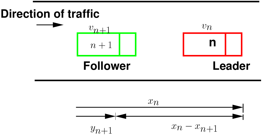
Before going in to the details, various notations used in car-following models are discussed here with the help of figure 1. The leader vehicle is denoted as n and the following vehicle as (n + 1). Two characteristics at an instant t are of importance; location and speed. Location and speed of the lead vehicle at time instant t are represented by xnt and vnt respectively. Similarly, the location and speed of the follower are denoted by xn+1t and vn+1t respectively. The following vehicle is assumed to accelerate at time t + ΔT and not at t, where ΔT is the interval of time required for a driver to react to a changing situation. The gap between the leader and the follower vehicle is therefore xnt - xn+1t.
The basic assumption of this model is “A good rule for following another vehicle at a safe distance is to allow yourself at least the length of a car between your vehicle and the vehicle ahead for every ten miles per hour of speed at which you are traveling” According to Pipe’s car-following model, the minimum safe distance headway increases linearly with speed. A disadvantage of this model is that at low speeds, the minimum headways proposed by the theory are considerably less than the corresponding field measurements.
In this model, the reaction time needed for the following vehicle to perceive the need to decelerate and apply the brakes is considered. That is, the time gap between the rear of the leader and the front of the follower should always be equal to or greater than the reaction time. Therefore, the minimum time headway is equal to the reaction time (minimum time gap) and the time required for the lead vehicle to traverse a distance equivalent to its length. A disadvantage of this model is that, similar to Pipe’s model, there is a wide difference in the minimum distance headway at low and high speeds.
The General Motors’ model is the most popular of the car-following theories because of the following reasons:
In car following models, the motion of individual vehicle is governed by an equation, which is analogous to the Newton’s Laws of motion. In Newtonian mechanics, acceleration can be regarded as the response of the particle to stimulus it receives in the form of force which includes both the external force as well as those arising from the interaction with all other particles in the system. This model is the widely used and will be discussed in detail later.
The concept of this model is that each driver tries to achieve an optimal velocity based on the distance to the preceding vehicle and the speed difference between the vehicles. This was an alternative possibility explored recently in car-following models. The formulation is based on the assumption that the desired speed vndesired depends on the distance headway of the nth vehicle. i.e.vndesiredt = vopt(Δxnt) where vopt is the optimal velocity function which is a function of the instantaneous distance headway Δxnt. Therefore ant is given by
![t opt t t
an = [1∕τ][V (Δx n)- vn]](web0x.png) | (1) |
where  is called as sensitivity coefficient. In short, the driving strategy of nth vehicle is that, it
tries to maintain a safe speed which in turn depends on the relative position, rather than
relative speed.
is called as sensitivity coefficient. In short, the driving strategy of nth vehicle is that, it
tries to maintain a safe speed which in turn depends on the relative position, rather than
relative speed.
The basic philosophy of car following model is from Newtonian mechanics, where the acceleration may be regarded as the response of a matter to the stimulus it receives in the form of the force it receives from the interaction with other particles in the system. Hence, the basic philosophy of car-following theories can be summarized by the following equation
![[Response]n α [Stimulus]n](web2x.png) | (2) |
for the nth vehicle (n=1, 2, ...). Each driver can respond to the surrounding traffic conditions only by accelerating or decelerating the vehicle. As mentioned earlier, different theories on car-following have arisen because of the difference in views regarding the nature of the stimulus. The stimulus may be composed of the speed of the vehicle, relative speeds, distance headway etc, and hence, it is not a single variable, but a function and can be represented as,
 | (3) |
where fsti is the stimulus function that depends on the speed of the current vehicle, relative position and speed with the front vehicle.
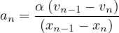
The car following model proposed by General motors is based on follow-the leader concept. This is based on two assumptions; (a) higher the speed of the vehicle, higher will be the spacing between the vehicles and (b) to avoid collision, driver must maintain a safe distance with the vehicle ahead.
Let Δxn+1t is the gap available for (n + 1)th vehicle, and let Δxsafe is the safe distance, vn+1t and vnt are the velocities, the gap required is given by,
 | (4) |
where τ is a sensitivity coefficient. The above equation can be written as
 | (5) |
Differentiating the above equation with respect to time, we get
![vtn - vtn+1 = τ.atn+1
1
atn+1 =--[vtn - vtn+1]
τ](web6x.png)
![[ ]
at = αl,m-(vtn+1)m- [vt- vt ]
n+1 (xtn - xtn+1)l n n+1](web7x.png) | (6) |
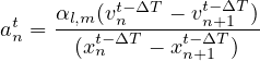
where l is a distance headway exponent and can take values from +4 to -1, m is a speed exponent and can take values from -2 to +2, and α is a sensitivity coefficient. These parameters are to be calibrated using field data. This equation is the core of traffic simulation models.
In computer, implementation of the simulation models, three things need to be remembered:
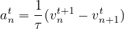
Therefore, the governing equations of a traffic flow can be developed as below. Let ΔT is the reaction time, and Δt is the updation time, the governing equations can be written as,
The equation 7 is a simulation version of the Newton’s simple law of motion v = u + at and equation 8 is the simulation version of the Newton’s another equation s = ut + at2. The
acceleration of the follower vehicle depends upon the relative velocity of the leader and the
follower vehicle, sensitivity coefficient and the gap between the vehicles.
at2. The
acceleration of the follower vehicle depends upon the relative velocity of the leader and the
follower vehicle, sensitivity coefficient and the gap between the vehicles.
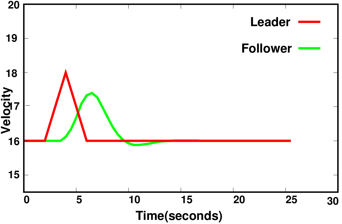
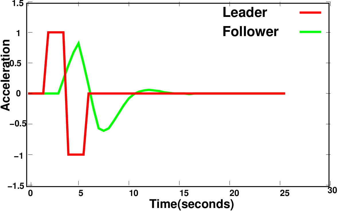
Let a leader vehicle is moving with zero acceleration for two seconds from time zero. Then he accelerates by 1 m∕s2 for 2 seconds, then decelerates by 1m∕s2for 2 seconds. The initial speed is 16 m/s and initial location is 28 m from datum. A vehicle is following this vehicle with initial speed 16 m/s, and position zero. Simulate the behavior of the following vehicle using General Motors’ Car following model (acceleration, speed and position) for 7.5 seconds. Assume the parameters l=1, m=0 , sensitivity coefficient (αl,m) = 13, reaction time as 1 second and scan interval as 0.5 seconds.
Solution
The first column shows the time in seconds. Column 2, 3, and 4 shows the acceleration,
velocity and distance of the leader vehicle. Column 5,6, and 7 shows the acceleration, velocity
and distance of the follower vehicle. Column 8 gives the difference in velocities between the
leader and follower vehicle denoted as dv. Column 9 gives the difference in displacement
between the leader and follower vehicle denoted as dx. Note that the values are assumed to
be the state at the beginning of that time interval. At time t=0, leader vehicle has a velocity of
16 m/s and located at a distance of 28 m from a datum. The follower vehicle is also
having the same velocity of 16 m/s and located at the datum. Since the velocity is
same for both, dv = 0. At time t = 0, the leader vehicle is having acceleration zero,
and hence has the same speed. The location of the leader vehicle can be found
out from equation as, x = 28+16×0.5 = 36 m. Similarly, the follower vehicle is not
accelerating and is maintaining the same speed. The location of the follower vehicle is, x =
0+16×0.5 = 8 m. Therefore, dx = 36-8 =28m. These steps are repeated till t = 1.5
seconds. At time t = 2 seconds, leader vehicle accelerates at the rate of 1 m∕s2
and continues to accelerate for 2 seconds. After that it decelerates for a period of
two seconds. At t= 2.5 seconds, velocity of leader vehicle changes to 16.5 m/s.
Thus dv becomes 0.5 m/s at 2.5 seconds. dx also changes since the position of
leader changes. Since the reaction time is 1 second, the follower will react to the
leader’s change in acceleration at 2.0 seconds only after 3 seconds. Therefore, at
t=3.5 seconds, the follower responds to the leaders change in acceleration given by
equation i.e., a =  = 0.23 m∕s2. That is the current acceleration of the follower
vehicle depends on dv and reaction time Δ of 1 second. The follower will change
the speed at the next time interval. i.e., at time t = 4 seconds. The speed of the
follower vehicle at t = 4 seconds is given by equation as v= 16+0.231×0.5 = 16.12
The location of the follower vehicle at t = 4 seconds is given by equation as x =
56+16×0.5+
= 0.23 m∕s2. That is the current acceleration of the follower
vehicle depends on dv and reaction time Δ of 1 second. The follower will change
the speed at the next time interval. i.e., at time t = 4 seconds. The speed of the
follower vehicle at t = 4 seconds is given by equation as v= 16+0.231×0.5 = 16.12
The location of the follower vehicle at t = 4 seconds is given by equation as x =
56+16×0.5+ ×0.231×0.52 = 64.03 These steps are followed for all the cells of the
table.
×0.231×0.52 = 64.03 These steps are followed for all the cells of the
table.
| t | a(t) | v(t) | x(t) | a(t) | v(t) | x(t) | dv | dx |
| (1) | (2) | (3) | (4) | (5) | (6) | (7) | (8) | (9) |
| t | a(t) | v(t) | x(t) | a(t) | v(t) | x(t) | dv | dx |
| 0.00 | 0.00 | 16.00 | 28.00 | 0.00 | 16.00 | 0.00 | 0.00 | 28.00 |
| 0.50 | 0.00 | 16.00 | 36.00 | 0.00 | 16.00 | 8.00 | 0.00 | 28.00 |
| 1.00 | 0.00 | 16.00 | 44.00 | 0.00 | 16.00 | 16.00 | 0.00 | 28.00 |
| 1.50 | 0.00 | 16.00 | 52.00 | 0.00 | 16.00 | 24.00 | 0.00 | 28.00 |
| 2.00 | 1.00 | 16.00 | 60.00 | 0.00 | 16.00 | 32.00 | 0.00 | 28.00 |
| 2.50 | 1.00 | 16.50 | 68.13 | 0.00 | 16.00 | 40.00 | 0.50 | 28.13 |
| 3.00 | 1.00 | 17.00 | 76.50 | 0.00 | 16.00 | 48.00 | 1.00 | 28.50 |
| 3.50 | 1.00 | 17.50 | 85.13 | 0.23 | 16.00 | 56.00 | 1.50 | 29.13 |
| 4.00 | -1.00 | 18.00 | 94.00 | 0.46 | 16.12 | 64.03 | 1.88 | 29.97 |
| 4.50 | -1.00 | 17.50 | 102.88 | 0.67 | 16.34 | 72.14 | 1.16 | 30.73 |
| 5.00 | -1.00 | 17.00 | 111.50 | 0.82 | 16.68 | 80.40 | 0.32 | 31.10 |
| 5.50 | -1.00 | 16.50 | 119.88 | 0.49 | 17.09 | 88.84 | -0.59 | 31.03 |
| 6.00 | 0.00 | 16.00 | 128.00 | 0.13 | 17.33 | 97.45 | -1.33 | 30.55 |
| 6.50 | 0.00 | 16.00 | 136.00 | -0.25 | 17.40 | 106.13 | -1.40 | 29.87 |
| 7.00 | 0.00 | 16.00 | 144.00 | -0.57 | 17.28 | 114.80 | -1.28 | 29.20 |
| 7.50 | 0.00 | 16.00 | 152.00 | -0.61 | 16.99 | 123.36 | -0.99 | 28.64 |
| 8.00 | 0.00 | 16.00 | 160.00 | -0.57 | 16.69 | 131.78 | -0.69 | 28.22 |
| 8.50 | 0.00 | 16.00 | 168.00 | -0.45 | 16.40 | 140.06 | -0.40 | 27.94 |
| 9.00 | 0.00 | 16.00 | 176.00 | -0.32 | 16.18 | 148.20 | -0.18 | 27.80 |
| 9.50 | 0.00 | 16.00 | 184.00 | -0.19 | 16.02 | 156.25 | -0.02 | 27.75 |
| 10.00 | 0.00 | 16.00 | 192.00 | -0.08 | 15.93 | 164.24 | 0.07 | 27.76 |
| 10.50 | 0.00 | 16.00 | 200.00 | -0.01 | 15.88 | 172.19 | 0.12 | 27.81 |
| 11.00 | 0.00 | 16.00 | 208.00 | 0.03 | 15.88 | 180.13 | 0.12 | 27.87 |
| 11.50 | 0.00 | 16.00 | 216.00 | 0.05 | 15.90 | 188.08 | 0.10 | 27.92 |
| 12.00 | 0.00 | 16.00 | 224.00 | 0.06 | 15.92 | 196.03 | 0.08 | 27.97 |
| 12.50 | 0.00 | 16.00 | 232.00 | 0.05 | 15.95 | 204.00 | 0.05 | 28.00 |
| 13.00 | 0.00 | 16.00 | 240.00 | 0.04 | 15.98 | 211.98 | 0.02 | 28.02 |
| 13.50 | 0.00 | 16.00 | 248.00 | 0.02 | 15.99 | 219.98 | 0.01 | 28.02 |
| 14.00 | 0.00 | 16.00 | 256.00 | 0.01 | 16.00 | 227.98 | 0.00 | 28.02 |
| 14.50 | 0.00 | 16.00 | 264.00 | 0.00 | 16.01 | 235.98 | -0.01 | 28.02 |
| 15.00 | 0.00 | 16.00 | 272.00 | 0.00 | 16.01 | 243.98 | -0.01 | 28.02 |
| 15.50 | 0.00 | 16.00 | 280.00 | 0.00 | 16.01 | 251.99 | -0.01 | 28.01 |
| 16.00 | 0.00 | 16.00 | 288.00 | -0.01 | 16.01 | 260.00 | -0.01 | 28.00 |
| 16.50 | 0.00 | 16.00 | 296.00 | 0.00 | 16.01 | 268.00 | -0.01 | 28.00 |
| 17.00 | 0.00 | 16.00 | 304.00 | 0.00 | 16.00 | 276.00 | 0.00 | 28.00 |
| 17.50 | 0.00 | 16.00 | 312.00 | 0.00 | 16.00 | 284.00 | 0.00 | 28.00 |
| 18.00 | 0.00 | 16.00 | 320.00 | 0.00 | 16.00 | 292.00 | 0.00 | 28.00 |
| 18.50 | 0.00 | 16.00 | 328.00 | 0.00 | 16.00 | 300.00 | 0.00 | 28.00 |
| 19.00 | 0.00 | 16.00 | 336.00 | 0.00 | 16.00 | 308.00 | 0.00 | 28.00 |
| 19.50 | 0.00 | 16.00 | 344.00 | 0.00 | 16.00 | 316.00 | 0.00 | 28.00 |
| 20.00 | 0.00 | 16.00 | 352.00 | 0.00 | 16.00 | 324.00 | 0.00 | 28.00 |
| 20.50 | 0.00 | 16.00 | 360.00 | 0.00 | 16.00 | 332.00 | 0.00 | 28.00 |
The earliest car-following models considered the difference in speeds between the leader and the follower as the stimulus. It was assumed that every driver tends to move with the same speed as that of the corresponding leading vehicle so that
 | (10) |
where τ is a parameter that sets the time scale of the model and  can be considered as a
measure of the sensitivity of the driver. According to such models, the driving strategy is to
follow the leader and, therefore, such car-following models are collectively referred to as the
follow the leader model. Efforts to develop this stimulus function led to five generations of
car-following models, and the most general model is expressed mathematically as
follows.
can be considered as a
measure of the sensitivity of the driver. According to such models, the driving strategy is to
follow the leader and, therefore, such car-following models are collectively referred to as the
follow the leader model. Efforts to develop this stimulus function led to five generations of
car-following models, and the most general model is expressed mathematically as
follows.
![t αl,m [vtn-+δ1t]m t-ΔT t-ΔT
an+1 = [xt-ΔT---xt-ΔT]l(vn - vn+1 )
n n+1](web14x.png) | (11) |
where l is a distance headway exponent and can take values from +4 to -1, m is a speed exponent and can take values from -2 to +2, and α is a sensitivity coefficient. These parameters are to be calibrated using field data.
The Greenberg’s stream model can be derived from General Motors car follwing model. The GM model is given as:
![t --αl,m-[vnt-+δ1t]m--- t-ΔT t-ΔT
an = [xt-nΔT - xtn-+Δ1T]l(vn - vn+1 )](web15x.png) | (12) |
Putting l = 1 and m = 0 the model becomes:
 | (13) |
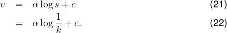
At steady state condtion, the equation becomes:
 | (14) |
Now integrating both sides with respect to tm we get:
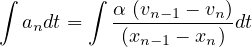 | (15) |
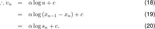
Now, put u = xn-1 - xn, then
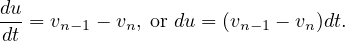 | (16) |
Therefore,


![ddqk- = α k [[ddkd-log kkj]+dα (log]kkj) ( k )
= α k ---logkj - --logk +α log-j
[dk ] ( dk ) k
= α k --1 + α log kj
k k
kj
= α log k - α = 0.
kj
∴ log k = 1,
kj kj
or k = e, or, k0 = e . (25)](web25x.png)
 | (27) |
Microscopic traffic flow modeling focuses on the minute aspects of traffic stream like vehicle to vehicle interaction and individual vehicle behavior. They help to analyze very small changes in the traffic stream over time and space. Car following model is one such model where in the stimulus-response concept is employed. Optimal models and simulation models were briefly discussed.
![[ ]
an+1(t) = 15× un(t-- 1)---un+1(t--1)
xn(t - 1) - xn+1(t- 1)](web28x.png) | (28) |
Modify the input file and use. To compile in linux use gcc prog.c -lm -o prog.exe and to run .\prog.exe.
I wish to thank several of my students and staff of NPTEL for their contribution in this lecture. I also appreciate your constructive feedback which may be sent to tvm@civil.iitb.ac.in
Prof. Tom V. Mathew
Department of Civil Engineering
Indian Institute of Technology Bombay, India
_________________________________________________________________________
Thursday 31 August 2023 12:13:06 AM IST
![vtn = vt-nδt+ atn-δt× δt (7)
xt = xt-δt+ vt-δt× δt+ 1at-δtδt2 (8)
n [n n ]2 n
t αl,m (vtn-+δ1t)m t-ΔT t- ΔT
an+1 = --t--ΔT---t-ΔT-l- (vn - vn+1 ) (9)
(xn - xn+1 )](web8x.png)