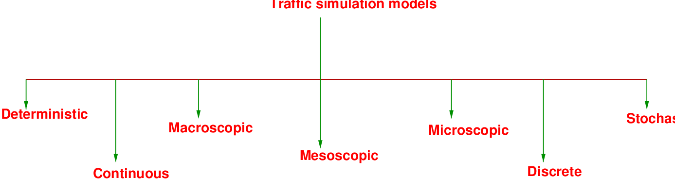
Figure 1: Classification of Traffic simulation models
The complexity of traffic stream behaviour and the difficulties in performing experiments with real world traffic make computer simulation an important analysis tool in traffic engineering. The physical propagation of traffic flows can be specifically described using traffic flow models. By making use of different traffic simulation models, one can simulate large scale real-world situations in great detail. Depending on the level of detailing, traffic flow models are classified into macroscopic, mesoscopic and microscopic models. Macroscopic models view the traffic flow as a whole whereas microscopic ones gives attention to individual vehicles and their interactions while the mesoscopic models fall in between these two. This chapter gives an overview of the basic concepts behind simulation models and elaboration about the microscopic approach for modelling traffic.
A microscopic model of traffic flow attempts to analyze the flow of traffic by modelling driver-driver and driver-road interactions within a traffic stream which respectively analyses the interaction between a driver and another driver on road and of a single driver on the different features of a road. Many studies and researches were carried out on driver’s behavior in different situations like a case when he meets a static obstacle or when he meets a dynamic obstacle. Among these, the pioneer development of car following theories paved the way for the researchers to model the behaviour of a vehicle following another vehicle in the 1950s and 1960s.
Simulation modelling is an increasingly popular and effective tool for analyzing a wide variety of dynamical problems those associated with complex processes which cannot readily be described in analytical terms. Usually, these processes are characterized by the interaction of many system components or entities whose interactions are complex in nature. Specifically, simulation models are mathematical/logical representations of real-world systems, which take the form of software executed on a digital computer in an experimental fashion. The most important advantage is that these models are by no means exhaustive.
Traffic simulation models have a large variety of applications in the required fields. Now-a-days they become inevitable tools of analysis and interpretation of real world situations especially in Traffic Engineering. The following are some situations where these models can find their scope.
It is important to note that simulation can only be used as an auxiliary tool for evaluation and extension of results provided by other conceptual or mathematical formulations or models.
Traffic simulations models can meet a wide range of requirements:
Traffic simulation models can be classified based on different criteria. Figure 1 shows various types of classification. In a broader sense, they can be categorized into continuous and discrete ones according to how the elements describing a system change their states. The latter is again classified into two.
The first, divides time into fixed small intervals and within each interval the simulation model computes the activities which change the states of selected system elements. For some specific applications, considerable savings in computational time can be achieved by the use of event based models where scanning is performed based on some abrupt changes in the state of the system (events). However the discrete time models could be a better choice where the model objectives require more realistic and detailed descriptions.
According to the level of detailing, simulation models can be classified into macroscopic, mesoscopic and microscopic models. A macroscopic model describes entities and their activities and interactions at a low level of detail. Traffic stream is represented in an aggregate measure in terms of characteristics like speed, flow and density. A mesoscopic model generally represents most entities at a high level of detail but describes their activities and interactions at a much lower level of detail. A microscopic model describes both the system entities and their interactions at a high level of detail. Car following models and lane changing models are some significant examples. The choice of a particular type of model depends on the nature of the problem of interest.
Depending on the type of processes represented by the model, there are deterministic and stochastic models. Models without the use of any random variables or in other words, all entity interactions are defined by exact mathematical/logical relationships are called deterministic models. Stochastic models have processes which include probability functions.
The basic steps involved in the development are same irrespective of the type of model. The different activities involved are the following.
The most significant steps among the above are described with the help of stating the procedure for developing a microscopic model.
The framework of a model consists of mainly three processes as mentioned below.
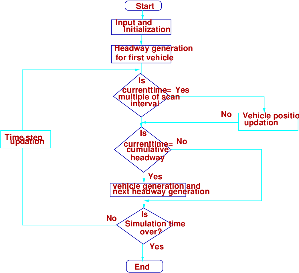
The flow diagram of a microscopic traffic simulation model is given in Figure 16.2. The basic structure of a model includes various component models like car following models like car following models, lane changing models etc. which come under the vehicle position updation part. In this chapter, the vehicle generation stage is explained in detail. The vehicles can be generated either according to the distributions of vehicular headways or vehicular arrivals. Headways generally follow one of the following distributions.
The generation of vehicles using negative exponential distribution is demonstrated here. The probability distribution function is given as follows.
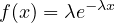 | (1) |
From the above equation, the expression for exponential variate headway X can be derived as:
 | (2) |
where, μ is the mean headway, R is the random number between 0 and 1
Random number generation is an essential part in any stochastic simulation model, especially in vehicle generation module. Numerous methods in terms of computer programs have been devised to generate random numbers which appear to be random. This is the reason why some call them pseudo-random numbers. Therefore headways can be generated using the above expression by giving a random number and the mean headway as the input variables.
In a similar way, the vehicular arrival pattern can be modeled using Poisson’s distribution. The probability mass function is given as:
 | (3) |
where, p(x) is the probability of x vehicle arrivals in an interval t, λ is the mean arrival rate of vehicles If the probability of no vehicle in the interval t is given as p(0), then this probability is same as the probability that the headway greater than or equal to t.
Given flow rate is 900 veh/hr. Simulate the vehicle arrivals for 1 min using negative exponential distribution.
Solution
Step 1: Calculate the mean headway μ =  = 4sec. Step 2: Generate the random
numbers between 0 and 1. Step 3: Calculate the headways and then estimate the cumulative
headways. The calculations are given in Table 1
= 4sec. Step 2: Generate the random
numbers between 0 and 1. Step 3: Calculate the headways and then estimate the cumulative
headways. The calculations are given in Table 1
 |
| Veh. No. | R | X | Arrival time (sec) |
| 1 | 0.73 | 1.23 | 1.23 |
| 2 | 0.97 | 0.14 | 1.37 |
| 3 | 0.27 | 5.26 | 6.63 |
| 4 | 0.44 | 3.25 | 9.88 |
| 5 | 0.52 | 2.63 | 12.51 |
| 6 | 0.77 | 1.05 | 13.55 |
| 7 | 0.43 | 3.39 | 16.94 |
| 8 | 0.81 | 0.84 | 17.79 |
| 9 | 0.08 | 9.96 | 27.75 |
| 10 | 0.74 | 1.18 | 28.93 |
| 11 | 0.53 | 2.58 | 31.51 |
| 12 | 0.81 | 0.83 | 32.34 |
| 13 | 0.15 | 7.46 | 39.80 |
| 14 | 0.44 | 3.26 | 43.06 |
| 15 | 0.29 | 5.02 | 48.08 |
| 16 | 0.68 | 1.56 | 49.63 |
| 17 | 0.05 | 12.09 | 61.72 |
The hourly flow rate in a road section is 900 veh/hr. Use Poisson distribution to model this vehicle arrival for 10 min.
Solution Step 1: Calculate the no. of vehicles arriving per min. λ = 900/60 = 15 veh/min. Step 2: Calculate the probability of 0, 1, 2, ... vehicles per minute using Poisson distribution formula. Also calculate the cumulative probability as shown below.
 |
Step 3: Generate random numbers from 0 to 1. Using the calculated cumulative probability values, estimate the no. of vehicles arriving in that interval as shown in Table below.
| n | p(x=n) | p(x¡=n) |
| 0 | 0.000 | 0 |
| 1 | 0.000 | 0.000 |
| 2 | 0.000 | 0.000 |
| 3 | 0.000 | 0.000 |
| 4 | 0.001 | 0.001 |
| 5 | 0.002 | 0.003 |
| 6 | 0.005 | 0.008 |
| 7 | 0.010 | 0.018 |
| 8 | 0.019 | 0.037 |
| 9 | 0.032 | 0.070 |
| 10 | 0.049 | 0.118 |
| 11 | 0.066 | 0.185 |
| 12 | 0.083 | 0.268 |
| 13 | 0.096 | 0.363 |
| 14 | 0.102 | 0.466 |
| 15 | 0.102 | 0.568 |
| 16 | 0.096 | 0.664 |
| 17 | 0.085 | 0.749 |
| 18 | 0.071 | 0.819 |
| 19 | 0.056 | 0.875 |
| 20 | 0.042 | 0.917 |
| t (min) | R | n |
| 1 | 0.231 | 11 |
| 2 | 0.162 | 10 |
| 3 | 0.909 | 19 |
| 4 | 0.871 | 18 |
| 5 | 0.307 | 12 |
| 6 | 0.008 | 6 |
| 7 | 0.654 | 15 |
| 8 | 0.775 | 17 |
| 9 | 0.632 | 15 |
| 10 | 0.901 | 20 |
| 143 | ||
Here the total number of vehicles arrived in 10 min is 143 which is almost same as the vehicle arrival rate obtained using negative exponential distribution.
The activity of specifying data to the model that describes traffic operations and other features which are site specific is called calibration of the model. In other words, calibration is the process of quantifying model parameters using real-world data. This data may take the form of scalar elements and of statistical distributions. Calibration is a major challenge during the implementation stage of any model. The commonly used methods of calibration are regression, optimization, error determination, trajectory analysis etc. A brief description about various errors and their significance is presented in this section. The optimization method of calibration is also explained using the following example problem.
The parameters obtained in GM car-following model simulation are given in Table below. Field observed values of acceleration of follower is also given. Calibrate the model by finding the value of α. Assume l=1 and m=0. Use optimization method to solve the problem.
| Observed Acceleration (aobs) | Velocity difference, dv | Distance headway, dx |
| 0.23 | 1.5 | 29.13 |
| 0.46 | 1.88 | 29.97 |
| 0.67 | 1.16 | 30.73 |
| 0.82 | 0.32 | 31.10 |
Solution Step 1: Formulate the objective function (z).
 |
Step 2: Express aical in terms of α. As per GM model (since l=1 and m=0),
 |
Step 3: Therefore the objective function can be expressed as:
 |
Step 4: Since the above function is convex, differentiating and then equating to zero will give the solution (as stationary point is the global minimum). Differentiating with respect to and equating to zero,
 |
Then, value of α is obtained as 9.74.
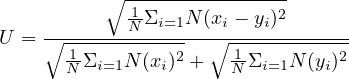
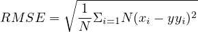
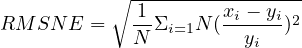
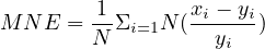
Most of the available commercial traffic simulation software provides advanced user-friendly graphic user interfaces with flexible and powerful graphic editors to assist analysts in the model-building process. This reduces the number of errors. There are a number of manual ways to quantify the error associated with every parameter while calibrating them. Some of the common measures of error and their expressions are discussed below.
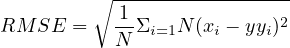 | (4) |
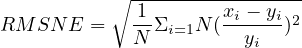 | (5) |
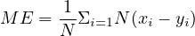 | (6) |
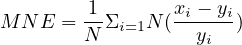 | (7) |
where, xi is the ith measured or simulated value, yi is the ith observed value
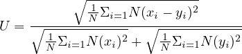
The above error measures are useful when applied separately to measurements at each location instead of to all measurements jointly. They indicate the existence of systematic bias in terms of under or over prediction by the simulation model. Taking into account that the series of measurements and simulated values can be collected at regular time intervals, it becomes obvious that they can be interpreted as time series and, therefore, used to determine how close the simulated and the observed values are. Thus it can be determined that how similar both time series are. On the other hand, the use of aggregated values to validate a simulation seems contradictory if one takes into account that it is dynamic in nature, and thus time dependent. Theil defined a set of indices aimed at this goal and these indices have been widely used for that purpose. The first index is Theil’s indicator, U (also called Theil’s inequality coefficient), which provides a normalized measure of the relative error that reduces the impact of large errors:
 | (8) |
The global index U is bounded, 0 ≤ U ≤ 1, with U = 0 for a perfect fit and xi = yi for i = 1 to N, between observed and simulated values. For U ≤ 0.2, the simulated series can be accepted as replicating the observed series acceptably well. The closer the values are to 0, the better will be the model. For values greater than 0.2, the simulated series is rejected.
The observed and simulated values obtained using Model 1 and Model 2 are given in Table below.
Simulated values, x | ||
| Observed values, y | Model 1 | Model 2 |
| 0.23 | 0.2 | 0.27 |
| 0.46 | 0.39 | 0.5 |
| 0.67 | 0.71 | 0.65 |
| 0.82 | 0.83 | 0.84 |
 |
 |
 |
 |
Tabulations required are given below.
| (x - y) | ( ) ) | (x - y)2 | ( )2 )2 |
| -0.030 | -0.130 | 0.0009 | 0.0170 |
| -0.070 | -0.152 | 0.0049 | 0.0232 |
| 0.040 | 0.060 | 0.0016 | 0.0036 |
| 0.010 | 0.012 | 0.0001 | 0.0001 |
| ϵ = -0.050 | ϵ = -0.211 | ϵ = 0.0075 | ϵ = 0.0439 |
| ME = 0.013 | MNE = 0.053 | RMSE = 0.043 | RMSNE = 0.105 |
| (x - y) | ( ) ) | (x - y)2 | ( )2 )2 |
| 0.040 | 0.174 | 0.0016 | 0.0302 |
| 0.040 | 0.087 | 0.0016 | 0.0076 |
| -0.020 | -0.030 | 0.0004 | 0.0009 |
| 0.020 | 0.024 | 0.0004 | 0.0006 |
| ϵ = 0.080 | ϵ = 0.255 | ϵ= 0.0040 | ϵ = 0.0393 |
| ME = 0.020 | MNE = 0.064 | RMSE = 0.032 | RMSNE = 0.099 |
Comparing Model 1 and Model 2 in terms of RMSE and RMSNE, Model 2 is better. But with respect to ME and MNE, Model 1 is better.
 |
The additional tabulations required are as follows:
| x2 | ||
| Model 1 | Model 2 | y2 |
| 0.04 | 0.0729 | 0.0529 |
| 0.1521 | 0.25 | 0.2116 |
| 0.5041 | 0.4225 | 0.4489 |
| 0.6889 | 0.7056 | 0.6724 |
| ϵ = 1.3851 | ϵ = 1.451 | ϵ = 1.3858 |
The value of Theil’s indicator is obtained as: For Model 1, U = 0.037 which is ≤ 0.2, and For Model 2, U = 0.027 which is ≤ 0.2. Therefore both models are acceptable.
Following de-bugging, verification is a structured regimen to provide assurance that the software performs as intended. Since simulation models are primarily logical constructs, rather than computational ones, the analyst must perform detailed logical path analyses. When completed, the model developer should be convinced that the model is performing in accord with expectations over its entire domain of application.
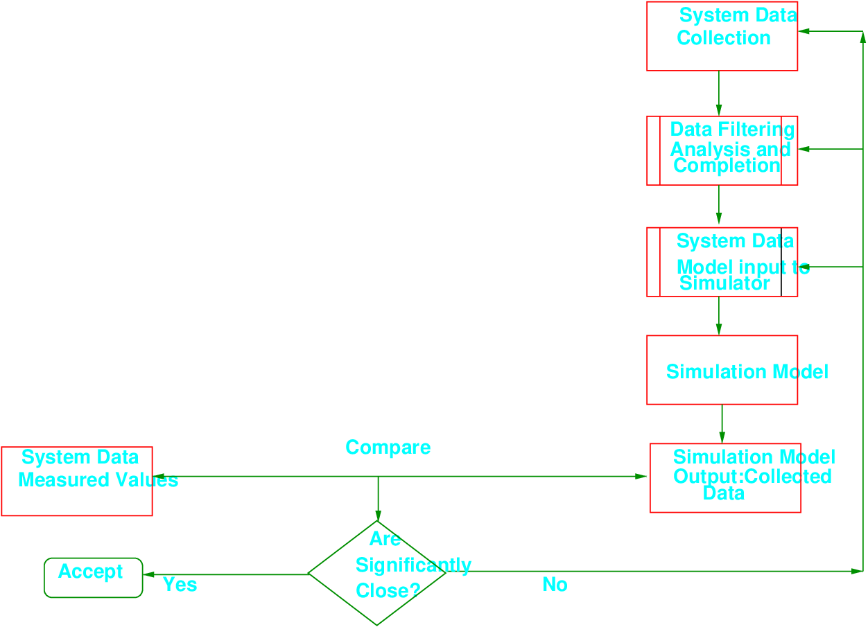
Validation is the process to determine whether the simulation model is an accurate representation of the system under study. This establishes that the model behaviour accurately and reliably represents the real-world system being simulated, over the range of conditions anticipated and it involves the following major steps.
The methodological scheme for validation is shown in the following Figure 3.
Now a days, traffic simulation packages like CORSIM and VISSIM are frequently used as tools for analyzing traffic. VISSIM is a microscopic, time step and behaviour based simulation model developed to analyze the full range of functionally classified roadways and public transportation operations. Since all these are commercial software packages, it is not possible to make sufficient changes in the internal parameters used in these models according to the specific requirements. Common applications of these packages include freeway and arterial corridor studies, sub-area planning studies, evacuation planning, freeway management strategy development, environmental impact studies, Intelligent Transportation Systems (ITS) assessments, current and future traffic management schemes etc.
Results of simulation can be interpreted in different ways. Animation displays of extracting the sought information and insights from the mass of the traffic environment (if available) are a most powerful tool for analyzing simulation results. If the selected traffic simulation lacks an animation feature or if questions remain after viewing the animation, then the following procedures may be adopted:
Statistical analysis of the simulation results are also conducted to present point estimates of effectiveness and to form the confidence intervals. Through these processes, one can establish that which simulation system is the best among the different alternatives.
It can be observed from the study that using different microscopic simulation models, large scale real-world situations can be simulated in great detail. New applications of traffic simulation can contribute significantly to various programs in ITS. Calibration and validation are the major challenges to be tackled. It is expected that further exploration would open up better opportunities for better utilization and further development of these models.
I wish to thank several of my students and staff of NPTEL for their contribution in this lecture. I also appreciate your constructive feedback which may be sent to tvm@civil.iitb.ac.in
Prof. Tom V. Mathew
Department of Civil Engineering
Indian Institute of Technology Bombay, India
_________________________________________________________________________
Thursday 31 August 2023 12:13:24 AM IST