Traffic Flow Modeling Analogies

Lecture Notes in Transportation Systems Engineering

Prof. Tom V. Mathew

PDF for Online View or PDF for Print
(PDF for IITB students and is password protected)

1 Introduction
2 Model framework
2.1 Assumptions
2.2 Formulation
2.3 Derivation of the Conservation equation
3 Analytical Solution
3.1 Formulation
3.2 Method of Characteristics
3.3 Inference
4 Conclusion
Exercises
References
Acknowledgments

______________________________________________________________________

1 Introduction

If one looks into traffic flow from a very long distance, the flow of fairly heavy traffic appears like a stream of a fluid. Therefore, a macroscopic theory of traffic can be developed with the help of hydrodynamic theory of fluids by considering traffic as an effectively one-dimensional compressible fluid. The behaviour of individual vehicle is ignored and one is concerned only with the behaviour of sizable aggregate of vehicles. The earliest traffic flow models began by writing the balance equation to address vehicle number conservation on a road. In fact, all traffic flow models and theories must satisfy the law of conservation of the number of vehicles on the road.

2 Model framework

2.1 Assumptions

The traffic flow is similar to the flow of fluids and the traffic state is described based on speed, density and flow. However the traffic flow can be modelled as a one directional compressible fluid. The two important assumptions of this modelling approach are:

The traffic flow is conserved, or in other words vehicles are not created or destroyed. The continuity or conservation equation can be applied.
There is one to one relationship between speed and density as well as flow and density.

The difficulty with this assumption is that although intuitively correct, in some cases this can lead to negative speed and density. Further, for a given density there exists many speed values are actually measured. These assumptions are valid only at equilibrium condition, that is, when the speed is a function of density. However, equilibrium can be rarely observed in practice and therefore hard to get Speed-density relationship. These are some of the limitations of continuous modelling. The advantages of the continuous modelling are:

Better than input output models because flow and density are set as a function of time and distance.
Compressibility: ie., flow is assumed to be a function of density.
Solving the continuity equation (or flow conservation equation) and the state equation (speed-density and flow-density) are basic traffic flow equations (q = k.v). By using the equation that define q, k, and v at any location x and time t, we can evaluate the system using measures of effectiveness such as delays, travel time etc.

2.2 Formulation

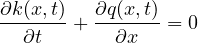
Assuming that the vehicles are flowing from left to right, the continuity equation can be written as

∂k(x,t) ∂q(x,t) --∂t---+ --∂x---= 0

(1)

where x denotes the spatial coordinate in the direction of traffic flow, t is the time, k is the density and q denotes the flow. However, one cannot get two unknowns, namely k(x,t) by and q(x,t) by solving one equation. One possible solution is to write two equations from two regimes of the flow, say before and after a bottleneck. In this system the flow rate before and after will be same, or

k1v1 = k2v2

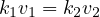(2)

From this the shock wave velocity can be derived as

q2 - q1 v(to)p = k---k-- 2 1

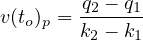(3)

This is normally referred to as Stock’s shock wave formula. An alternate possibility which Lighthill and Whitham adopted in their landmark study is to assume that the flow rate q is determined primarily by the local density k, so that flow q can be treated as a function of only density k. Therefore the number of unknown variables will be reduced to one. Essentially this assumption states that k(x,t) and q (x,t) are not independent of each other. Therefore the continuity equation takes the form

∂k (x,t) ∂q(k(x,t)) -------+ ---------= 0 ∂t ∂x

(4)

However, the functional relationship between flow q and density k cannot be calculated from fluid-dynamical theory. This has to be either taken as a phenomenological relation derived from the empirical observation or from microscopic theories. Therefore, the flow rate q is a function of the vehicular density k; q = q(k). Thus, the balance equation takes the form

∂k-(x,t) ∂q(k(x,t))- ∂t + ∂x = 0

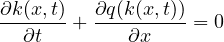(5)

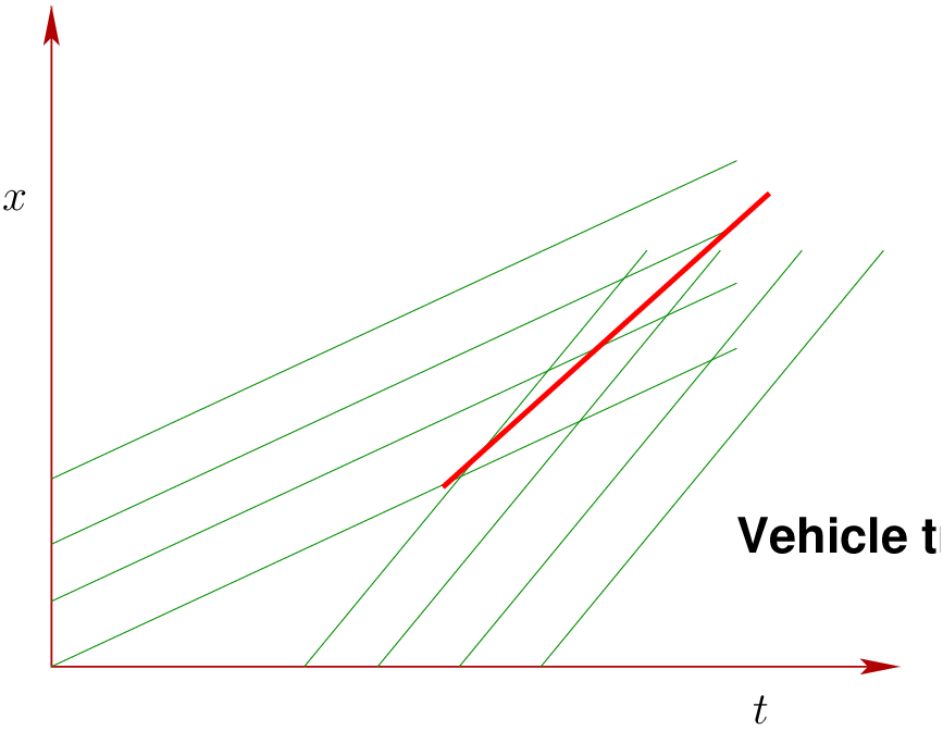
Now there is only one independent variable in the balance equation, the vehicle density k. If initial and boundary conditions are known, this can be solved. Solution to LWR models are kinematic waves moving with velocity

dq(k) dk

(6)

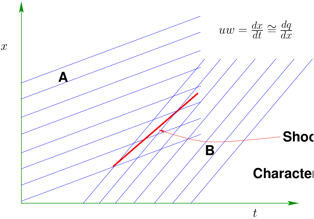
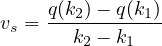
This velocity v_k is positive when the flow rate increases with density, and it is negative when the flow rate decreases with density. In some cases, this function may shift from one regime to the other, and then a shock is said to be formed. This shock wave propagate at the velocity

q(k2)- q(k1) vs = --k---k---- 2 1

(7)

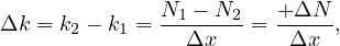
where q(k₂) and q(k₁) are the flow rates corresponding to the upstream density k₂ and downstream density k₁ of the shock wave. Unlike Stock’s shock wave formula there is only one variable here.

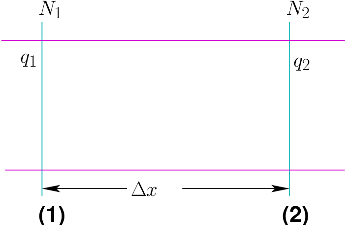
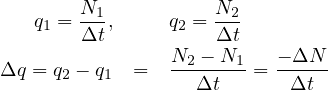
2.3 Derivation of the Conservation equation

Consider a unidirectional continuous road section with two counting station.

Figure 1: CAP

Let N₁ : number of cars passing (1) in time Δt; q₁ : the flow; N₂ : number of cars passing (2) in time Δt; and q₂ : the flow; Assume N₁ > N₂, then queuing between (1) and (2)

q1 = N1-, q2 = N2- Δt Δt Δq = q2 - q1 = N2 --N1-= - ΔN- Δt Δt

Note that q₂ < q₁ and therefore Δq is negative. Therefore,

ΔN = - Δq.Δt

(8)

Similarly (k₂ > k₁),

Δk = k2 - k1 = N1---N2-= +-ΔN-, Δx Δx

Therefore

ΔN = Δk Δx

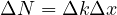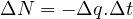
From the above two equations:

Δk Δx + Δq Δt = 0

Dividing by Δt Δx

Δk Δq --- + ---= 0 Δt Δx

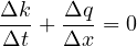Assuming continuous medium (ie., taking limits) lim_t→0

∂q- ∂k- ∂x + ∂t = 0

If sink or source is considered

∂q-+ ∂k-= g(x,t) ∂x ∂t

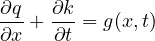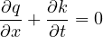
where, g(x,t) is the generation or dissipation term (Ramp on and off). Solution to the above was proposed by Lighthill and Whitham (1955) and Richard (1956) popularly knows as LWR Model.

3 Analytical Solution

3.1 Formulation

The analytical solution, popularly called as LWR Model, is obtained by defining the relationship between the fundamental dependant traffic flow variable (kandq) to the independent variable (xandt). However, the solution to the continuity equation needs one more equation: by assuming q = f(k) , ie., q = k.v. Therefore:

∂f ∂∂(kqx)-+ ∂∂∂ktk- = 0,becomes --∂k- + ∂t- = 0 ∂k ∂(k.v) ∂t-+ -∂x--- = 0 ∂k ∂[k.f(k)] ---+ -------- = 0,v = f(k) ∂t ∂x

Therefore,

∂[k.f(k)] ∂k- ∂f(k) ∂x = ∂x.f(k)+ k. ∂x ∂k- df-∂k- = ∂xf(k)+ k.dk.∂x ∂k-[ -df-] = ∂x f(k)+ k.dk

Continuity equation can be written as

∂∂kt + ∂∂kx [f(k)+ k.ddfk] = 0

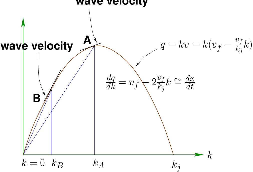
where f(k) could be any function relating density and speed. Eg: Assuming the Greenshield’s linear model:

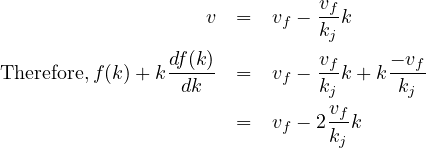
v v = vf --fk kj Therefore,f (k) +k df-(k)- = vf - vfk + k- vf- dk kj kj = v - 2vfk f kj

Therefore,

∂k- ∂k-[ vf ] ∂t + ∂x vf - 2kj k = 0

(9)

The equation 9 is first order quasi-linear, hyperbolic, partial differential equation (a special kind of wave equation).

3.2 Method of Characteristics

Consider k(x,t) at each point of x and t, and ∂k∂t + ∂∂kx [f(k) + ddfk k] = 0 in the total derivative of k along a curve which has slope ∂x
∂t = f(k) + df-
dk k. ie., Along any curve in (x,t), consider x,k as function of t.

Figure 2: aa

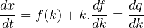
Total derivative of k will be

dk- ∂k- ∂k-dx- dt = ∂t + ∂x .[dt ] ∂k- ∂k- df- = ∂t + ∂x f(k)+ dk k

At the solution, dk-
dt

= 0, k is constant along the curve, f(k) + k. df-
dk

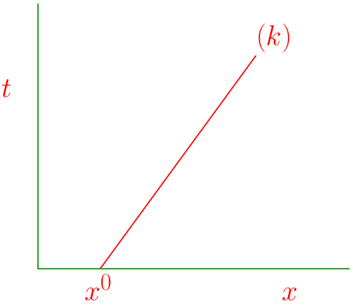
is constant along the curve. That is,

[ ] dx- x(t) = x0 + dt t [ dt] = x0 + f(k)+ k.---t dk

Note that the solution is to construct some curve e so that: (a) k_t + c(k).k_x is the total derivative of k along the curve (ie., directional derivative) and (b) slope of the curve dx
dt

= c(k). We know k(x,t). Therefore directional derivative k(x,t) along t

dk(x,t) = ∂k-+ dx-.∂k- dt ∂t d[t ∂x ] = ∂k-+ f(k)+ k.df- ∂k- ∂t dk ∂x = 0 dk- ie.,dt = 0

That is k is constant along the curve e or dx
dt

= f(k) + k -df
dk

is constant along curve e. Therefore e must be straight line.

[ ] x(t) = x0 + f(k )+ k.df- t dk

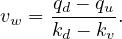
If k(x,0) = k₀ is initial condition

x(t) = x0 + [f(k0)+ k0.df|k=k0]t dk

This function is plotted below along with a fundamental q-k diagram.

Figure 3: AA

Figure 4: BB

Figure 5: CC

3.3 Inference

Density k is constant along characteristic lines
Characteristic lines are straight lines emanating from the boundaries of x-t plane
The slope of the characteristic line is
$dx-= f(k)+ k.df-≡ dq- dt dk dk$
ie., Characteristic curve has the slope equal to the tangent of the flow density curve.
When two Characteristic lines intersect (ie., 2 k values at a given x,t) shock waves are generated; and characteristic line terminate.
Shock wave represent mathematical discontinuity ie., abrupt changes to k,q,v.
Speed of the Shock wave is ratio of the time storage rate to space storage rate; that is:
$vw = qd --qu. kd - kv$

4 Conclusion

The advantages of the continuous modelling is that it gives good insight into the understanding of the behaviour of traffic. It can also be applied to platoon movement, signal control, etc. Finally, it also paves the way for the development of higher order models. However, it also has some serious limitations. The first one is the difficulty in getting solutions for realistic problems(initial boundary conditions). Second, the q - k and u - k relationship are complex. It may also cause unrealistic abrupt changes in the system. Finally acceleration-deceleration characteristics are not directly modelled in the system.

Exercises

Write a brief note on the shockwave phenomenon and illustrate with neat sketches.
Explain the shock-wave phenomenon and derive the expression for speed of a shock wave with the help of neat diagrams.
Derive the flow conservation equation for a mid-block section.
Derive the LWR formulation of traffic flow if we assume Greenshilds linear model relating speed and density.
Illustrate the method of characteristics for solving an LWR formulation.
Derive the numerical formulation to solve an LWR formulation using finite difference method. Illustrate the scheme also.
(i) Derive the hyperbolic (explicit) form of LWR model using the following parameters in Greenshield’s equation. Free flow speed is 80 kmph; Jam density is 320 veh/hr. (ii) Find the values of density at points (t=0.25 hr, x=15 km) and (t=1.0 hr, x=70 km) using the method of characteristics with the following initial condition:
${ 80 veh∕km if 0 < x ≤ 10 km k(x,0) = k0(x) 60 veh∕km if 0 > 10 km (10 )$

References

D Chowdhury, L Santen, and A Schadschneider. Statistical physics of vehicular traffic and some related systems. Physics Report 329, 2000. 199-329.
L R Kadiyali. Traffic Engineering and Transportation Planning. Khanna Publishers, New Delhi, 1987.

Acknowledgments

I wish to thank several of my students and staff of NPTEL for their contribution in this lecture. I also appreciate your constructive feedback which may be sent to tvm@civil.iitb.ac.in

Prof. Tom V. Mathew
Department of Civil Engineering
Indian Institute of Technology Bombay, India

_________________________________________________________________________

Thursday 31 August 2023 01:03:36 AM IST