Contents

1 Introduction

Models are necessary to simulate the real world scenario to some extent, or in some cases, they can even provide the exact scenario. Characteristics of traffic changes with time, place, human behavior etc. The models in traffic engineering are necessary to predict the behavior of traffic in proper planning and design of the road network. The models can be microscopic and macroscopic. In the present chapter, a macroscopic model has been discussed known as cell transmission model which tries to simulate the traffic behavior.

In the classical methods to explain macroscopic behaviour of traffic, like hydrodynamic theory, differential equations need to be solved to predict traffic evolution. However in situations of sudden high density variations, like bottle-necking, the hydrodynamic model calls for a shock wave (an ad-hoc). Hence these equations are essentially piecewise continuous which are difficult to solve. Cell transmission models are developed as a discrete analogue of these differential equations in the form of difference equations which are easy to solve and also take care of high density changes.

In this lecture note the hydrodynamic model and cell transmission model and their equivalence is discussed. The cell transmission model is explained in two parts, first with only a source and a sink, and then it is extended to a network. In the first part, the concepts of basic flow advancement equations of CTM and a generalized form of CTM are presented. In addition, the phenomenon of instability is also discussed. In the second segment, the network representation and topologies are established, after which the model is discussed in terms of a linear program formulation for merging and diverging.

2 Single source and sink CTM model

2.1 Basic Premise

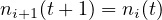
The cell transmission model simulates traffic conditions by proposing to simulate the system with a time-scan strategy where current conditions are updated with every tick of a clock. The road section under consideration is divided into homogeneous sections called cells, numbered from i = 1 to I. The lengths of the sections are set equal to the distances travelled in light traffic by a typical vehicle in one clock tick. Under light traffic condition, all the vehicles in a cell can be assumed to advance to the next with each clock tick. i.e,

(1)

where, n_i(t) is the number of vehicles in cell i at time t. However, equation 1 is not reasonable when flow exceeds the capacity. Hence a more robust set of flow advancement equations are presented in a later section.

2.2 Flow Advancement Equations

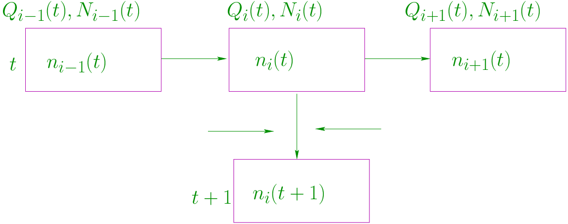
First, two constants associated with each cell are defined, they are: (i) N_i(t) which is the maximum number of vehicles that can be present in cell i at time t, it is the product of the cell’s length and its jam density. (ii) Q_i(t) : is the maximum number of vehicles that can flow into cell i when the clock advances from t to t + 1 (time interval t), it is the minimum of the capacity of cells from i - 1 and i. It is called the capacity of cell i. It represents the maximum flow that can be transferred from i - 1 to i. We allow these constants to vary with time to be able to model transient traffic incidents. Now the flow advancement equation can be written as, the cell occupancy at time t + 1 equals its occupancy at time t, plus the inflow and minus the outflow; i.e.,

(2)

where, n_i(t + 1) is the cell occupancy at time t + 1, n_i(t) the cell occupancy at time t, y_i(t) is the inflow at time t, y_i+1(t) is the outflow at time t. The flows are related to the current conditions at time t as indicated below:

(3)

where, n_i-1(t): is the number of vehicles in cell i- 1 at time t, Q_i(t): is the capacity flow into i for time interval t, N_i(t) - n_i(t): is the amount of empty space in cell i at time t.

Figure 1: Flow advancement

2.3 Boundary conditions

Boundary conditions are specified by means of input and output cells. The output cell, a sink for all exiting traffic, should have infinite size (N_I+1 = ∞) and a suitable, possibly time-varying, capacity. Input flows can be modeled by a cell pair. A source cell numbered 00 with an infinite number of vehicles (n₀₀(O) = ∞) that discharges into an empty gate cell 00 of infinite size, N₀(t) = ∞. The inflow capacity Q₀(t) of the gate cell is set equal to the desired link input flow for time interval t + 1.

2.4 Equivalence with Hydrodynamic theory

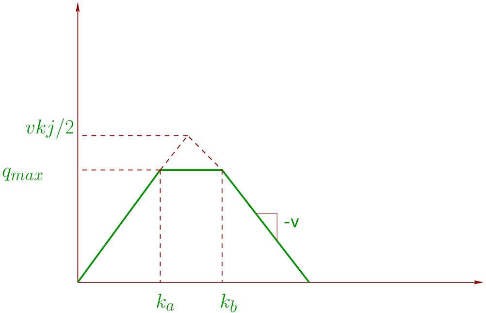
Consider equations 2 &  3, they are discrete approximations to the hydrodynamic model with a density- flow (k-q) relationship in the shape of an isoscaled trapezoid, as in Fig.2. This relationship can be expressed as:

(4)

Flow conservation is given by,

(5)

To demonstrate the equivalence of the discrete and continuous approaches, the clock tick set to be equal to ∂t and choose the unit of distance such that v∂t = 1. Then the cell length is 1, v is also 1, and the following equivalences hold: x ≡ i, k_j ≡ N, q_max ≡ Q, and k(x,t) ≡ n_i(t) with these conventions, it can be easily seen that the equations 4 &  3 are equivalent. Equation 6 can be equivalently written as:

(6)

This represents change in flow over space equal to change in occupancy over time. Rearranging terms of equation 7 we can arrive at equation 3, which is the same as the basic flow advancement equation of the cell transmission model.

Figure 2: Flow-density relationship for the basic cell-transmission model

3 Generalized CTM

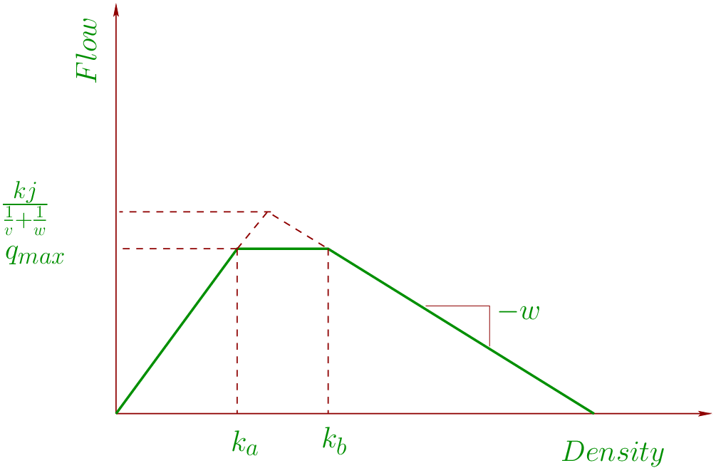
Generalized CTM is an extension of the cell transmission model that would approximate the hydrodynamic model for an equation of state that allows backward waves with speed w ≤ v (see Fig. 3 ). This is a realistic model, since on many occasions speed of backward wave will not be same as the free flow speed.

Figure 3: Flow-density relationship for the generalized CTM

(7)

A small modification is made in the above equation to avoid the error caused due to numerical spreading. Equation 7 is rewritten as

(8)

where, α = 1 if n_i-1(t)  ≤  Q_i(t), and α = w∕v if n_i-1(t)  >  Q_i(t).

3.1 Numerical example

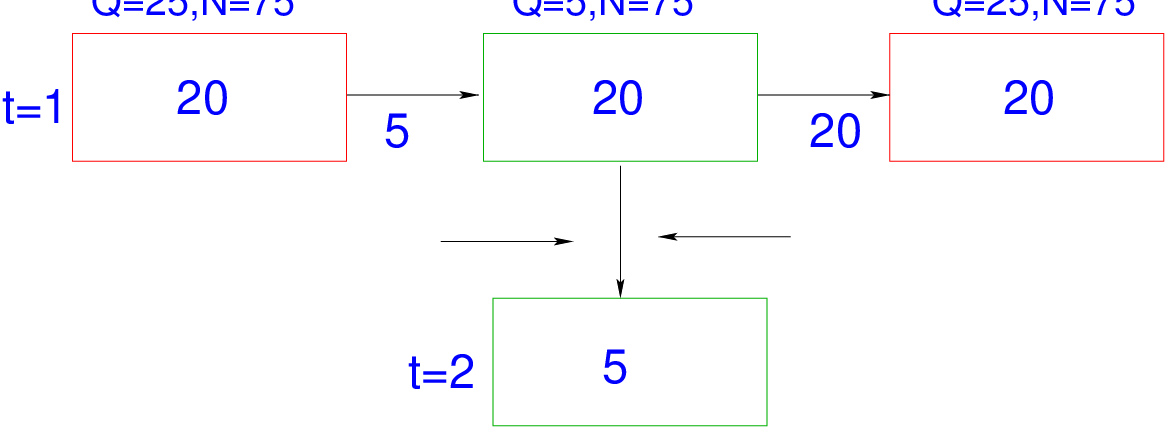
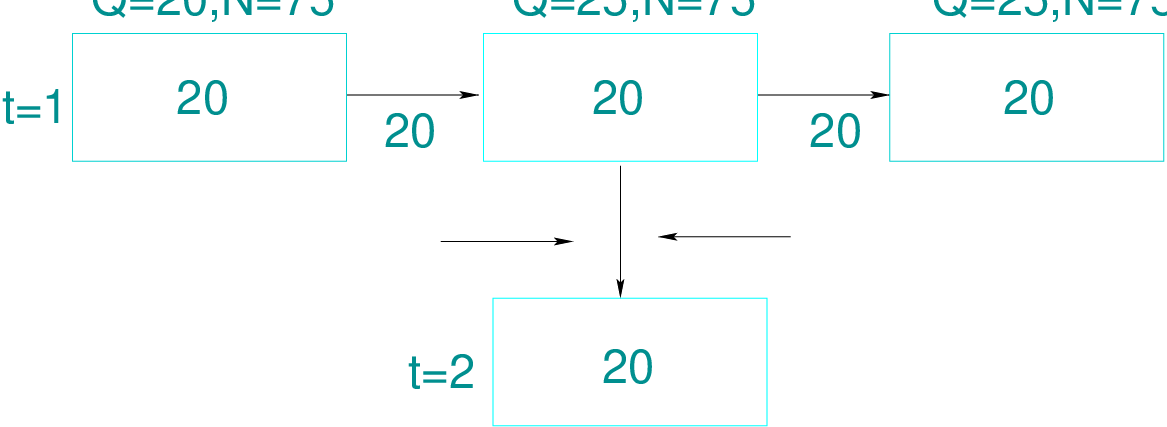
Consider a 1.25 km homogeneous road with speed v = 50 kmph, jam density k_j = 180 veh∕km and q_max = 3000 veh∕hr. Initially traffic is flowing undisturbed at 80% of capacity: q = 2400 veh∕hr. Then, a partial lane blockage lasting 2 min occurs on 1∕3^rd of the distance from the end of the road. The blockage effectively restricts flow to 20% of the maximum. Clearly, a queue is going to build and dissipate behind the restriction. After 2 minutes, the flow in cell 3 is maximum possible flow. Predict the evolution of the traffic. Take one clock tick as 30 seconds.

Solution The main purpose of cell transmission model is to simulate the real traffic conditions for a defined stretch of road. The speed and cell length is kept constant and also the cell lengths in cell transmission model. The solution has been divided into 4 steps as follows:

Step 1: Determination of cell length and number of cells Given clock tick, t = 30sec = 1∕120^th of an hour. So, cell length = distance travelled by vehicle in one clock tick = v × t = 50 × (1∕120) ≈ 5∕12 km. Road stretch given = 1.25 km. Therefore, no of cells = 1.25∕(5∕12) = 3 cells

Step 2: Determination of constants (N & Q) N = maximum number of vehicles that can be at time t in cell i, = cell length x jam density, = 180 x (5/12) = 75 vehicles, Q = maximum number of vehicles that can flow into cell I from time t to t+1, = 3000 x (1/120) = 25 vehicles. Now, to simulate the traffic conditions for some time interval, our main aim is to find the occupancies of the 3 cells (as calculated above) with the progression of clock tick. This is easily showed by creating a table. First of all, the initial values in the tables are filled up.

Step 3: Determination of cell capacity in terms of number of vehicles for various traffic flows. For 20% of the maximum = 600 × (1∕120) vehicles. For 80% of the maximum = 2400 × (1∕120) vehicles.

Step 4: Initialization of the table The table has been prepared with source cell as a large capacity value and a gate is there which connects and regulates the flow of vehicles from source to cell 1 as per the capacity of the cell for a particular interval. The cell constants (Q and N) for the 3 cells are shown in the table. Note that the sink can accommodate maximum number of vehicles whichever the cell 3 generates. Q3 is the capacity in terms of number of vehicles of cell 3 . The value from H5 to H7 (i.e 5) corresponds to the 2min time interval with 4 clock ticks when the lane was blocked so the capacity reduced to 20% of the maximum (i.e. 600 × (1/120)  vehicles). After the 2 min time interval is passed vehicles flows with full capacity in cell 3. So the value is 25 (i.e 3000 × (1/120) vehicles).

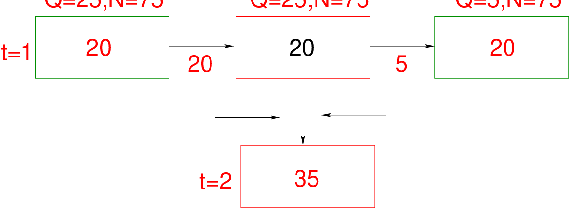
Step 5: Computation of Occupancies Simulation need not be started in any specific order, it can be started from any cell in the row corresponding to the current clock tick. Now, consider cell circled (cell 2 at time 2) in the final table. Its entry depends on the cells marked with rectangles. By flow conservation law: Occupancy = Storage + Inflow - Outflow. Note that the Storage is the occupancy of the same cell from the preceding clock tick. Also outflow of one cell is equal to the inflow of the just succeeding cell. Here, Storage = 20. For inflow use equation 3 Inflow= min [20,25,(75-20)]= 20. Outflow= min [20,5,(75-20)]= 5. Occupancy= 20+20-5=35.

Figure 4: ...

Now, For cell 1 at time 2, Inflow= min [20,min(25,25),(75-20)]= 20, Outflow= min [20,min(25,20),(75-20)]= 20, Occupancy= 20+20-20=20.

Now, For cell 3 at time 2, Inflow= min [20, min (25,5),(75-20)]= 5. Outflow= 20 (:.sink cell takes all the vehicles in previous cell) Occupancy= 20+5-20=5.

Figure 5:

Similarly, rest of the entries can be filled and the final result is shown in Table below.

From the table it can be seen that the occupancy i.e. the number of vehicles on cell 1 and 2 increases and then decreases simulating the effect of lane blockage in cell 3 on cell 1 and cell 2. The lane blockage lasts 2 minutes in this problem, after that there is no congestion taken into account. So as the time passes by, the occupancy in cell 1 and cell 2 also gets reduced.

3.2 Numerical example

Consider a 1.25 km homogeneous road with speed v = 50 kmph, jam density k_j = 180 veh/km and q_max = 3000 veh/hr. Initially traffic is flowing undisturbed at 80% of capacity: q = 2400 VPH. Then, a partial lane blockage lasting 2 min occurs l/3 of the distance from the end of the road. The blockage effectively restricts flow to 20% of the maximum. Clearly, a queue is going to build and dissipate behind the restriction. Predict the evolution of the traffic. Take one clock tick as 6 seconds.

Solution This problem is same as the earlier problem, only change being the clock tick. This problem has been solved in Excel.

The simulation is done for this smaller clock tick; the results are shown in Fig. 3 One can clearly observe the pattern in which the cells are getting updated. After the decrease in capacity on last one-third segment queuing is slowly building up and the backward wave can be appreciated through the first arrow. The second arrow shows the dissipation of queue and one can see that queue builds up at a faster than it dissipates. This simple illustration shows how CTM mimics the traffic conditions.

4 CTM: Network Traffic

4.1 General

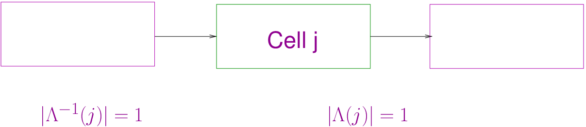
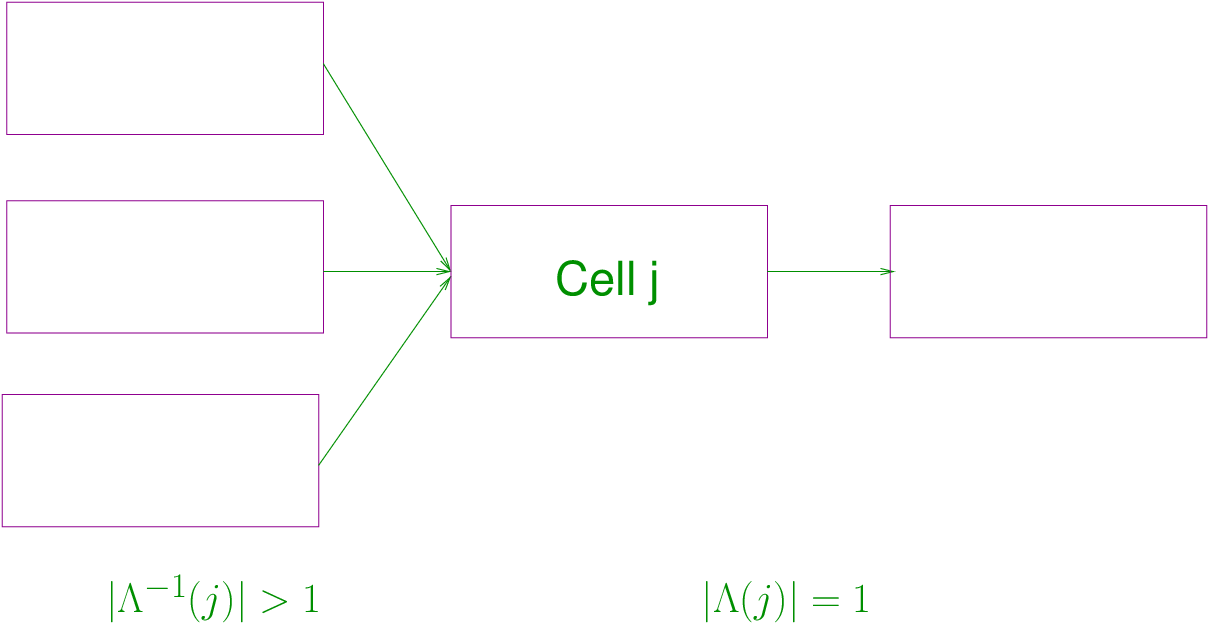
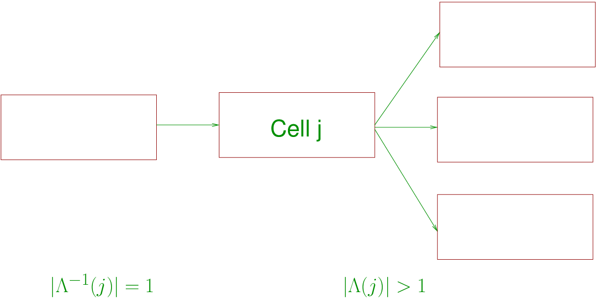
As sequel to his first paper on CTM, Daganzo (1995) published first paper on CTM applied to network traffic. In this section application of CTM to network traffic considering merging and diverging is discussed. Some basic notations: (The notations used from here on, are adopted from Ziliaskopoulos (2000)) Γ^-1 = Set of predecessor cells. Γ = Set of successor cells.

4.2 Network topologies

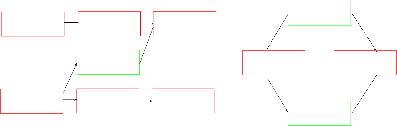
The notations introduced in previous section are applied to different types of cells, as shown in Figures 6, 7 &  8. Some valid and invalid representations in a network are shown in Fig 12 & Fig 11.

Figure 6: Source Cell

Figure 7: Sink Cell

Figure 8: Ordinary Cell

Figure 9: Merging Cell

Figure 10: Diverging Cell

Figure 11: Invalid representations

Figure 12: Valid representations

4.3 Ordinary link

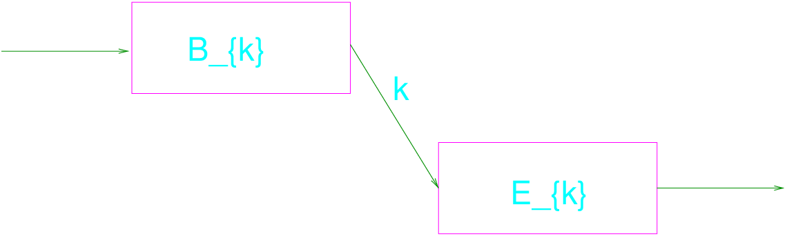
Consider an ordinary link with a beginning cell and ending cell, which gives the flow between two cells is simplified as explained below.

Figure 13: Ordinary Link

(9)

where, δ = w∕v. y_k(t) is the inflow to cell Ek in the time interval (t,t + 1). Defining the maximum flows that can be sent and received by the cell i in the interval between t to t + 1 as S_I(t) = min(QI,nI), and R_I(t) = min(Q_I,δ_I,[N_I -n_I]). Therefore, y_k(t) can be written in a more compact form as: y_k(t) = min(S_Bk,R_Ek). This means that the flow on link k should be the maximum that can be sent by its upstream cell unless prevented to do so by its end cell. If blocked in this manner, the flow is the maximum allowed by the end cell. From equations one can see that a simplification is done by splitting y_k(t) in to S_Bk and R_Ek terms. ’S’ represents sending capacity and ’R’ represents receiving capacity. During time periods when S_Bk < R_Ek the flow on link k is dictated by upstream traffic conditions-as would be predicted from the forward moving characteristics of the Hydrodynamic model. Conversely, when S_Bk > R_Ek, flow is dictated by downstream conditions and backward moving characteristics.

4.4 Merging and Diverging

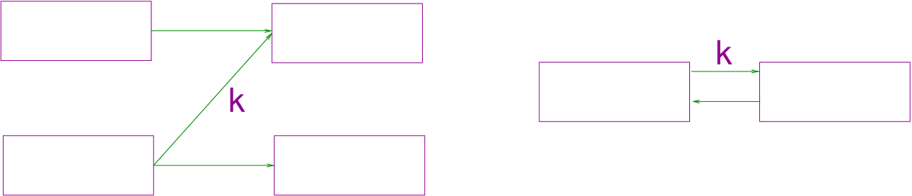
Consider two cells merging, here we have a beginning cell and its complimentary merging into ending cell, the constraints on the flow that can be sent and received are given by equation 10 and equation 10.

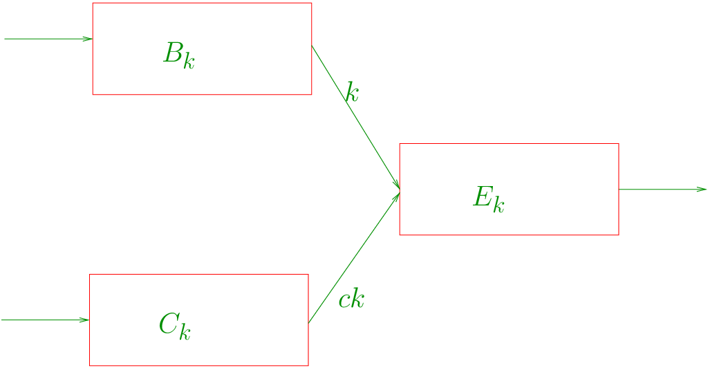
A number of combinations of y_k(t) + y_ck(t) are possible satisfying the above said constraints. Similarly for diverging a number of possible outflows to different links is possible satisfying corresponding constraints, hence this calls for an optimization problem. Ziliaskopoulos (2000), has given this LP formulations for both merging and diverging, this has been discussed later

5 CTM Software - NETCELL

1. NETCELL is a freeway network simulation program based on the cell transmission model developed by Cay ford, Lin and Daganzo.
2. It consists of two components,
   1. NETCELL
   2. NETVIEW(a graphical post-processor)
3. This is a free software and can be downloaded from the link below http://www.ce.berkeley.edu/ daganzo/software_and_data.htm
4. NETCELL is a macroscopic simulation program in which vehicle quantities are treated as continuous variables. Vehicles are advanced in a way consistent with the hydrodynamic theory of traffic flow.

6 Conclusion

6.1 Summary

1. CTM is a discrete approximation of hydrodynamic model. System evolution is based on difference equations.
2. Unlike hydrodynamic model, it explains the phenomenon of Instability.
3. Lesser the time per clock tick lesser are the size of cells and more accurate results would be obtained. But a compromise is needed between accuracy and computational effort. Largest possible cell size which would sufficiently give the details needed must be chosen.
4. CTM has many applications in DTA, NDP, traffic operations, emergency evacuations etc.
5. There is a vast scope for improvement and applications of this model.

6.2 Advantages and applications

1. CTM is consistent with hydrodynamic theory, which is a widely used model for studying macroscopic behavior of the traffic.
2. It is simple and sufficiently accurate for planning purposes.
3. CTM can be used to provide ”real time” information to the drivers.
4. CTM has been used in developing a system optimal signal optimization formulation.
5. CTM based Dynamic Traffic Assignment have shown good results.
6. CTM has its application in Network Design Problems.(NDP)

6.3 Limitations

1. CTM is for a ”typical vehicle” in network traffic, work is needed for the multi-modal representation of traffic.
2. Cell length cannot be varied. For this the methods like Modified Cell Transmission Model is to be used.
3. CTM is largely deterministic, stochastic variables are needed to be introduced to represent the random human behavior.

Exercises

1. Not Available

References

1. C D Alexandru. A stochastic mesoscopic cell transmission model for operational analysis of large-scale transportation networks. A dissertation submitted to Louisiana State University, 2006.
2. C F Daganzo. The cell transmission model Part I: A simple dynamic representation of highway traffic. Research Report UCB-ITS-PATH-RR-93-7, University of California, Berkeley, 1993.
3. C F Daganzo. The cell transmission model: A dynamic representation of highway traffic consistent with the hydrodynamic theory. Transportation Research B, 28(4):269-287, 1994.
4. C F Daganzo. The cell transmission model. Part II: Network Traffic. Transportation Research B, 29(2):79-93, 1995.
5. A K Ziliaskopoulos. A Linear Programming Model for the Single Destination System Optimum Dynamic Traffic Assignment Problem. Transportation Science, Vol.34,No. 1, 2000.

Acknowledgments

I wish to thank several of my students and staff of NPTEL for their contribution in this lecture. Specially, I wish to thank my student Mr. Pruthvi M, Mr. Varun for his assistance in developing the lecture note, and my staff Mr. Rayan in typesetting the materials. I also appreciate your constructive feedback which may be sent to tvm@civil.iitb.ac.in

Prof. Tom V. Mathew
Department of Civil Engineering
Indian Institute of Technology Bombay, India