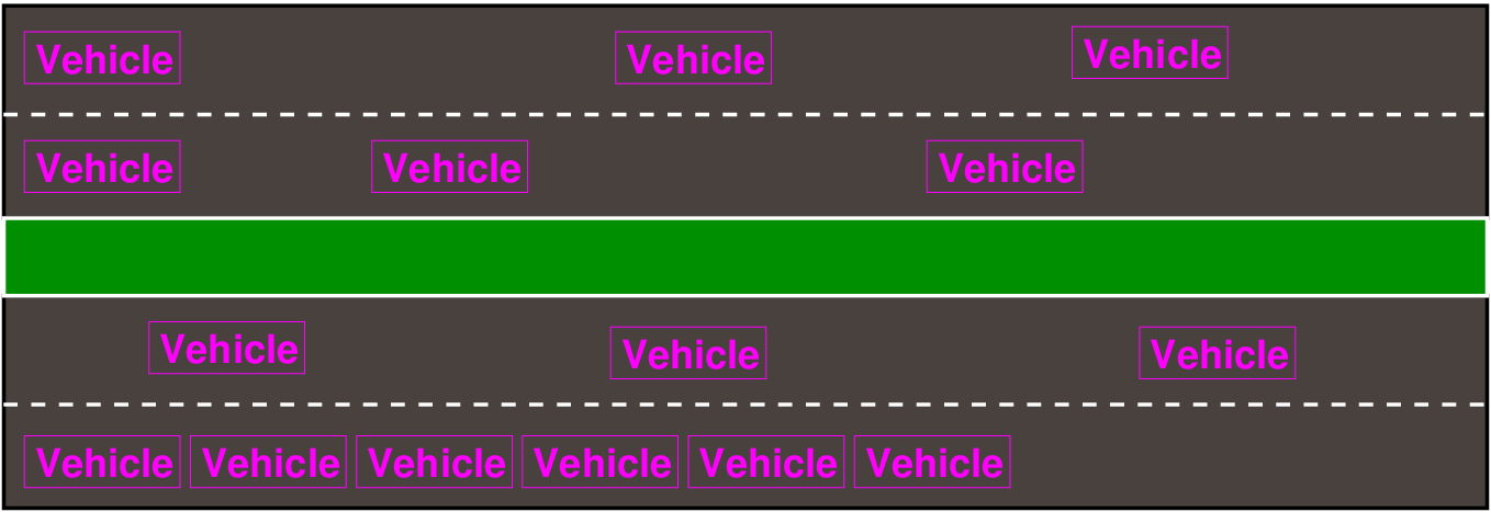
Figure 1: A vehicle Platoon
A majority of the metro cities in India are facing the problem of traffic congestion, delays, which have further resulted in pollution. The delays are caused mainly due to the isolated functioning of the traffic signals at closely located intersections. For better regulation of traffic flow at these intersections, the traffic signals need to be coordinated or linked. For the linking of signals, the vehicle movement characteristics from upstream signal to downstream signal need to be considered and simulated. Traffic Progression Models model the vehicle movement characteristics and help in the linking of signals. First, the concept of platoon, platoon variables is discussed and then platoon ratio is defined which is required for determination of arrival type. Then, the phenomenon of platoon dispersion and platoon dispersion model is introduced for understanding dispersion behavior of the vehicles. Finally, one of the platoon dispersion models i.e., Roberson’s platoon dispersion model is discussed, which estimates the vehicle arrivals at downstream locations based on an upstream departure profile.
A vehicle Platoon is defined as a group of vehicles travelling together. A vehicle Platoon is shown in Fig. 1.
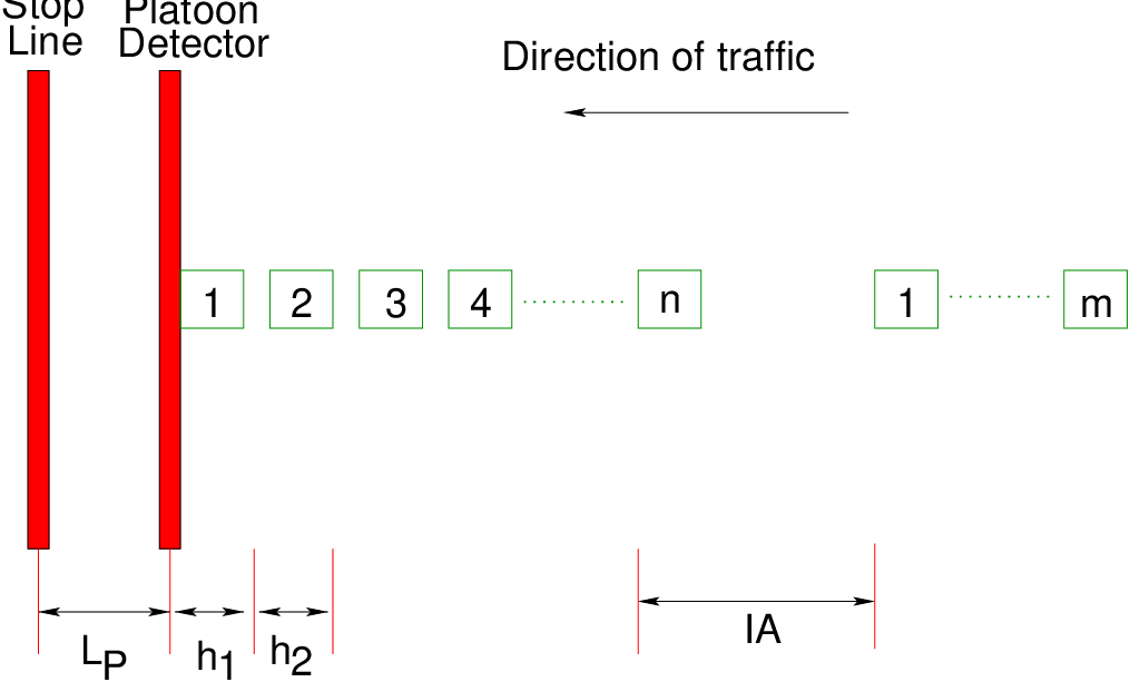
The various vehicle platoon characteristics or variables include platoon size, platoon headway, platoon speed and inter-arrival headway. Platoon behaviour and distribution patterns could be identified with respect to these parameters. The various platoon characteristics are illustrated in Fig. 2.
Various values of platoon headway and inter-arrival between consecutive platoons can be used to determine appropriate critical headway for platoon identification and detection. Once the critical headway is determined, platoon size and platoon speed can be detected to calculate the signal timing adjustment to accommodate the approaching vehicle platoon. It is of great importance to select a proper value of the critical headway since a small change in the critical headway will generate tremendous changes in the resultant platoon characteristics. Use of a large critical headway will result in a large average platoon size and require a large detection area in order to detect large vehicle platoons. Consequently, a large detection area leads to an increase of detector installation and maintenance costs. On the other hand, use of a small critical headway will result in a small average platoon size, but may not provide sufficient vehicle platoon information. Therefore, it is desired to find an appropriate critical headway so that sufficient platoon information can be obtained within a proper detection area. Research has shown that headways are rarely less than 0.5 seconds or over 10 seconds at different traffic volumes. Many investigations have been done on finding the effects of critical headways of 1.2, 1.5, 2.1 and 2.7 seconds on platoon behaviour and these investigations have shown that a critical headway of 2.1 seconds corresponding to a traffic volume of 1500 vehicles per hour per lane (vphpl) can be taken for data collection.
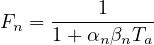
The platoon ratio denoted as Rp, is a numerical value used to quantify the quality of progression on an approach. The platoon ratio represents the ratio of the number of vehicles arriving during the green phase to the proportion of the green interval of the total cycle. This is given by
 | (1) |
where, P = Proportion of all vehicles during green time, C = Cycle length, g = Effective green time. Its value ranges from 0.5 to 2.0. It is used in the calculation of delays, capacity of an approach. The arrival types range from 1 (worst platoon condition) to 6 (the best platoon condition). The platoon ratio approximates the arrival type and the progression quality. For example HCM (2000) has suggested the following relationship between platoon ratio and arrival which is as shown in Table 1.
| Arrival | Range of platoon | Default value(Rp) | Progression quality |
| type | ratio(Rp) | ||
| 1 | ≤ 0.50 | 0.333 | Very poor |
| 2 | > 0.50 - 0.85 | 0.667 | Unfavorable |
| 3 | > 0.85 - 1.15 | 1.000 | Random arrivals |
| 4 | > 1.15 - 1.50 | 1.333 | Favorable |
| 5 | > 1.5 - 2.00 | 1.667 | Highly favorable |
| 6 | > 2 | 2.000 | Exceptional |
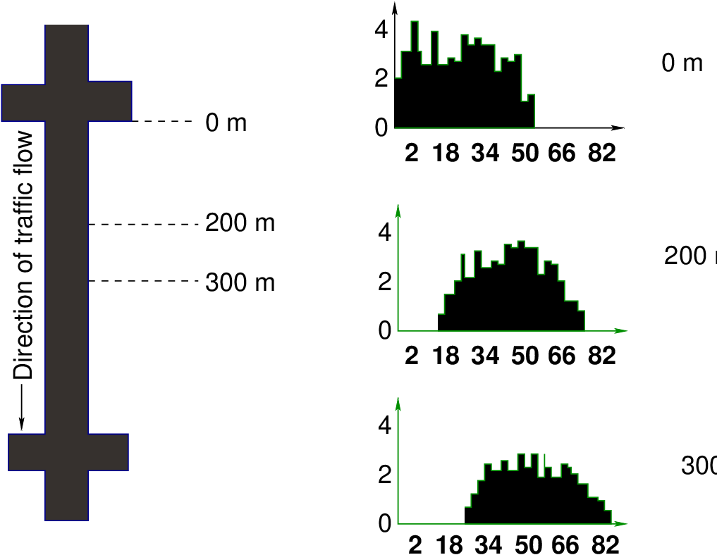
As a platoon moves downstream from an upstream intersection, the vehicles disperse i.e., the distance between the vehicles increase which may be due to the differences in the vehicle speeds, vehicle interactions (lane changing and merging) and other interferences (parking, pedestrians, etc.,). This phenomenon is called as Platoon Dispersion.
Dispersion has been found to be a function of the travel time from a signal to a downstream signal (or other downstream location) and the length of the platoon. The longer the travel time between signals, the greater the dispersion. This is intuitively logical since the longer the travel time, the more time (opportunity) there is for different drivers to deviate from the average travel time. A simple case of Platoon Dispersion is as shown in Fig. 3. From the figure, it can be observed that, initially the peak of the platoon is high and the length of the platoon is comparatively small, but as the platoon progresses downstream, the peak of the platoon decreases and the length increases.
Various traffic engineering software like TRANSYT (Traffic Network Study Tool) and SCOOT (Split Cycle Offset Optimization Technique) have employed the phenomenon of Platoon Dispersion for the prediction of Arrival Types. A flow profile obtained from TRANSYT-7F is as shown in the Fig. 4. From this figure also, it can be observed that, initially the peak of the platoon is high and the length of the platoon is small, but as the platoon progresses downstream, the peak of the platoon decreases and the length increases.
Platoon dispersion models simulate the dispersion of a traffic stream as it travels downstream by estimating vehicle arrivals at downstream locations based on an upstream vehicle departure profile and a desired traffic-stream speed. There are two kinds of mathematical models describing the dispersion of the platoon, namely:
One of the geometric distribution models is the Robertson’s platoon dispersion model, which has become a virtually universal standard platoon dispersion model and has been implemented in various traffic simulation software. Research has already been conducted on the applicability of platoon dispersion as a reliable traffic movement model in urban street networks. Most of the research has shown that Robertson’s model of platoon dispersion is reliable, accurate, and robust.
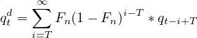
The basic Robertson’s recursive platoon dispersion model takes the following mathematical form
 | (2) |
where, qtd= arrival flow rate at the downstream signal at time t, qt-T= departure flow rate at the upstream signal at time t-T, T = minimum travel time on the link (measured in terms of unit steps T =βTa), Ta = average link travel time, n = modeling time step duration, Fn is the smoothing factor given by:
 | (3) |
αn = platoon dispersion factor (unit less) βn = travel time factor (unit less) Equation shows that the arrival flows in each time period at each intersection are dependent on the departure flows from other intersections. Note that the Robertson’s platoon dispersion equation means that the traffic flow qtd, which arrives during a given time step at the downstream end of a link, is a weighted combination of the arrival pattern at the downstream end of the link during the previous time step qt-nd and the departure pattern from the upstream traffic signal T seconds ago qt-T.
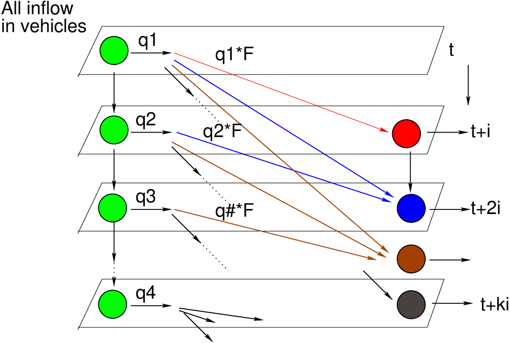
Fig. 5 gives the graphical representation of the model. It clearly shows that predicated flow rate at any time step is a linear combination of the original platoon flow rate in the corresponding time step (with a lag time of t) and the flow rate of the predicted platoon in the step immediately preceding it. Since the dispersion model gives the downstream flow at a given time interval, the model needs to be applied recursively to predict the flow. Seddon developed a numerical procedure for platoon dispersion. He rewrote Robertson’s equation as,
 | (4) |
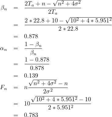
This equation demonstrates that the downstream traffic flow computed using the Robertson’s platoon dispersion model follows a shifted geometric series, which estimates the contribution of an upstream flow in the (t - i)th interval to the downstream flow in the tth interval. A successful application of Robertson’s platoon dispersion model relies on the appropriate calibration of the model parameters. Research has shown that the travel-time factor (βn) is dependent on the platoon dispersion factor (αn). Using the basic properties of the geometric distribution of Equation 5, the following equations have been derived for calibrating the parameters of the Robertson platoon dispersion model.
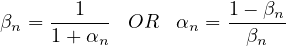 | (5) |
Equation 5 demonstrates that the value of the travel time factor (β) is dependent on the value of the platoon dispersion factor (α) and thus a value of 0.8 as assumed by Robertson results in inconsistencies in the formulation. Further, the model requires calibration of only one of them and the other factors can be obtained subsequently.
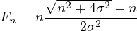
 | (6) |
where, σ is the standard deviation of link travel times and Ta is the average travel time between upstream and downstream intersections. Equation demonstrates that travel time factor can be obtained knowing the average travel time, time step for modeling and standard deviation of the travel time on the road stretch.
 | (7) |
Equation 7 further permits the calculation of the smoothing factor directly from the standard deviation of the link travel time and time step of modeling. Thus, both βn and Fn can be mathematically determined as long as the average link travel time, time step for modeling and its standard deviation are given.
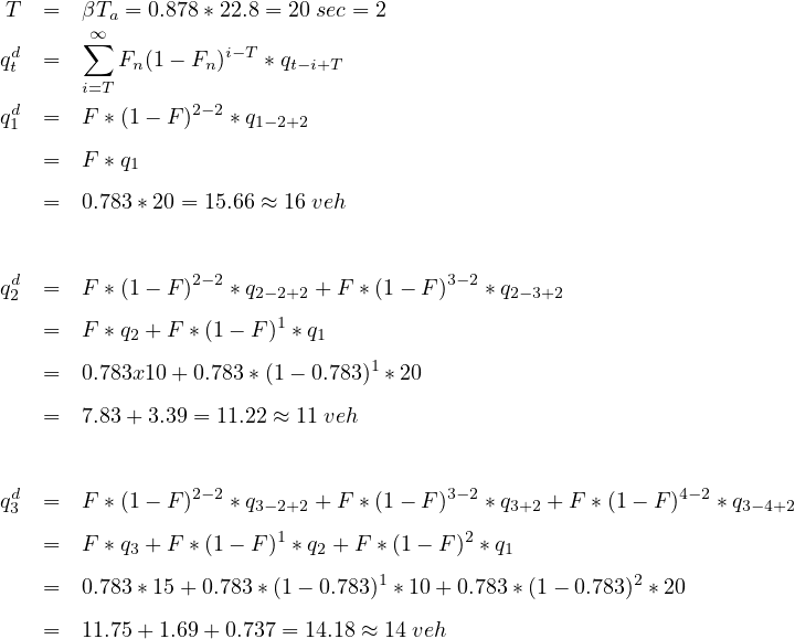
In a case study, the average travel time for a particular stretch was found out to be 22.8 seconds, standard deviation is 5.951 and model time step duration is 10 sec. Find out the Robertson’s model parameters and also the flow at downstream at different time steps where the upstream flows are as given as: q10 sec = 20,q20 sec = 10,q30 sec = 15,q40 sec = 18,q50 sec = 14,q60 sec = 12.
Solution Given, The model time step duration n=10sec, average travel time (Ta)=22.8sec, standard deviation (σ)=5.951. From equations above.
Upstream Flows: Since the modelling time step duration is given as n=10 sec, the given upstream flows can be written as follows:
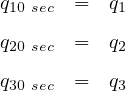
Downstream Flows: On the downstream, at 10 sec the flow will be zero since the modelling step duration is 10 sec. Hence the downstream flows can be written as follows.
In a case study, the average travel time from the upstream point to 1st downward point (point in between upstream and downstream) was found out to be 22.8 seconds and from upstream point to downward point (end point) was found out to be 32.8 seconds , standard deviation is 5.951 and model time step duration is 10 sec. Find out the Robertson’s model parameters and also the flow at downstream at different time steps where the upstream flows are as given below. q10 sec = 20,q20 sec = 10,q30 sec = 15,q40 sec = 18,q50 sec = 14,q60 sec = 12.
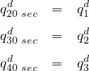
Solution This problem is similar to the earlier problem. Only there are 2 downstream points given in this. For the first downstream point, upstream values of flow given in the problem will be used, whereas for the 2nd downstream point, the flow from the 1st downstream point is to be used. Hence at 1st downstream point, flow in the first interval is zero and at the 2nd downstream value, flow is zero for first 2 intervals. The calculations have been done in excel and the following shows the results.
| Upstream Vol. for (in sec.) | No. of Vehicles |
| 10 | 20 |
| 20 | 10 |
| 30 | 15 |
| 40 | 18 |
| 50 | 14 |
| 60 | 12 |
| 0 | |
| 0 | |
| 0 | |
| 0 | |
| 89 | |
| Smoothing Factor F | 0.783 |
| Lag Time(For In Between Point) | 20 sec |
| Lag Time(For End Point) | 30 sec |
| Downstream Volume | Downstream Volume | ||
| At in between Point | At End Point | ||
| (in seconds) | (in seconds) | ||
| 10 | 0 | 10 | 0.00 |
| 20 | 15.66 | 20 | 0.00 |
| 30 | 11.23 | 30 | 12.26 |
| 40 | 14.18 | 40 | 11.45 |
| 50 | 17.17 | 50 | 13.59 |
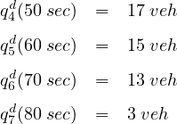
| 60 | 14.69 | 60 | 16.39 |
| 70 | 12.58 | 70 | 15.06 |
| 80 | 2.73 | 80 | 13.12 |
| 90 | 0.59 | 90 | 4.99 |
| 100 | 0.13 | 100 | 1.55 |
| 0.00 | 110 | 0.44 | |
| 88.96 | 120 | 0.09 | |
| 88.84 | |||
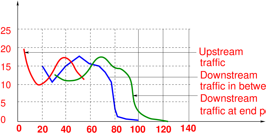
Four graphs are plotted below. The first graph shows the upstream profile, the second shows the downstream profile at in between point, the third shows the downstream profile at the end point. The last graph shows the comparison of all the three.
Initially, the concept of platoon and platoon variables was discussed. The platoon variables are required for the determination of critical headway which further helps in platoon identification. Then, the platoon ratio was defined which helps us in identifying the arrival type. Later, platoon dispersion model was discussed which model the departure profile of the downstream vehicles based on the upstream departure profile. Finally, Robertson’s platoon dispersion model is discussed with the help of numerical examples. The Robertson’s platoon dispersion model estimates the downstream volume at different time intervals which can be used for the linking of the signals and optimization of signal timings.
I wish to thank several of my students and staff of NPTEL for their contribution in this lecture.
I wish to thank my student Mr. Chetan Kumar and Ms. K Sravya for their assistance in developing the lecture note, and my staff Mr. Rayan in typesetting the materials. I also wish to thank several of my students and staff of NPTEL for their contribution in this lecture. I also appreciate your constructive feedback which may be sent to tvm@civil.iitb.ac.in
Prof. Tom V. Mathew
Department of Civil Engineering
Indian Institute of Technology Bombay, India
_________________________________________________________________________
Thursday 31 August 2023 01:04:10 AM IST