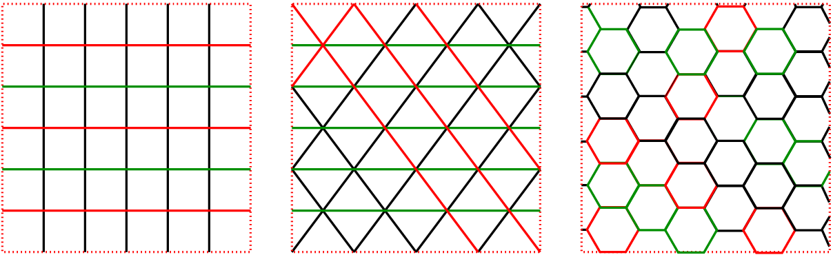
Figure 1: Physical environment as different types of cells
Traditional microscopic traffic simulation involves models that describe the behaviour of individual vehicles at every instant of time and every location of the road. Hence, such models are complex as they try to capture the behaviour in detailed way and are therefore time consuming especially for large networks. Cellular Automata is a new paradigm in traffic flow modeling and simulation which proposes computationally efficient and robust framework. The main advantage was an efficient and fast performance when used in computer simulations without significant compromise on accuracy for large scale applications. The traffic cellular automata (TCA) are dynamical systems that are discrete in nature, in the sense that time advances with discrete steps and space is coarse-grained. This chapter presents the basics of cellular automta and details of how CA concepts are used in traffic simulation.
A Cellular Automata is an n-dimensional array of simple cells where each cell may be in any one of k-states. At each tick of the clock a cell will change its state based on the states of the cells in a local neighborhood. Typically, the rule for updating the state does not change over time, and is applied to the whole grid simultaneously. Due to its simplicity the CA rules are used to solve the complex behaviour. Through the use of powerful computers, these models can encapsulate the complexity of the real world traffic behavior and produces clear physical patterns that are similar to those we see in everyday life. One more advantage of cellular automata models is their efficiency in showing the clear transition from the moving traffic to jamming traffic. CA models have the distinction of being able to capture micro-level dynamics and relate these to macro level traffic flow behavior.
There are four components which play a major role in cellular automata, namely, the physical environment, the state of the cell, the neighbourhood, and a local transition rule. These are explained below.
The term physical environment indicates the physical platform on which CA is computed. It normally consists of discrete lattice of cells with rectangular, hexagonal etc shown in Fig. 1. All these cells are equal in size. They can be finite or infinite in size and its dimensionality can be 1 (a linear string of cells called an elementary cellular automaton or ECA).
Every cell can be in a particular state where typically an integer can determine the number of distinct states a cell can be in, eg (binary state). Generally, the cell is assigned with an integer value or a null value based upon its state. The states of cells collectively are called as “Global configuration”. This convention clearly indicates that states are local and refer to cells, while a configuration is global and refers to the whole lattice.
The future state of a cell is mainly dependent on its state of its neighbourhood cell, so neighbourhood cell determines the evolution of the cell. So generally, the lattices vary as one-dimensional and two-dimensional. In one dimensional lattice, the present cell and the two adjacent cells forms its neighbourhoods ( shown in Fig. 2), whereas in the context of two dimensional lattice there are four adjacent cells which acts as the neighbourhoods. Therefore, it is clear that as the dimensionality increases the no of adjacent
cells also increases.
This rule (also called function) acts upon a cell and its direct neighbourhood, such that the cell’s state changes from one discrete time step to another (i.e., the system’s iterations). The CA evolves in time and space as the rule is subsequently applied to all the cells in parallel. Typically, the same rule is used for all the cells (if the converse is true, then the term hybrid CA is used). When there are no stochastic components present in this rule, we call the model a deterministic CA, as opposed to a stochastic (also called probabilistic) CA.
When the cellular automaton analogy is applied to vehicular road traffic flows, the physical environment of the system represents the road on which the vehicles are been driving. In a general single-lane setup for traffic cellular automata, this layout consists of a one-dimensional lattice that is composed of individual cells (the description here mainly focuses on unidirectional, single-lane traffic). Every cell either can be empty, or occupied by exactly one vehicle. We use the term single-cell models to describe these systems. Multi-cell models are those models, where the vehicle has a possibility to span several consecutive cells. Because vehicles move from one cell to another, TCA models are also called particle-hopping models.
An example of the tempo-spatial dynamics of such a system is depicted in the below Fig.4, where two consecutive vehicles i and j are driving on a one-dimensional lattice. Here we assume T = 1 s and X = 7.5m, corresponding to speed increments of V =X/T =27 km/h. The spatial discretisation corresponds to the average length a conventional vehicle occupies in a closely jam packed (and as such, its width is neglected), whereas the temporal discretisation is based on a typical driver’s reaction time and we implicitly assume that a driver does not react to events between two consecutive time steps.
In traffic stream, the movement of the individual vehicles is described by means of a rule set that reflects the car-following and lane-changing behaviour of a traffic cellular automaton evolving in time and space. The TCAs local transition rule actually comprises this set of rules. These rules are applied to all the vehicles in parallel (where in that case it is called as parallel update). Therefore, in a classic setup, the system’s state is changed through synchronous position updates of all the vehicles.
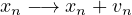
For each vehicle, the new speed is computed, after which its position is updated according to this speed and a possible lane-change manoeuvre. Note that there are other ways to perform this update procedure, e.g., a random sequential update. It is assumed that a driver does not react to events between consecutive time steps. For single-lane traffic, we assume that vehicles act as anisotropic particles, i.e., they only respond to frontal stimuli. So typically, the car-following part of a rule set only considers the direct frontal neighbourhood of the vehicle to which the rules are applied.
The radius of this neighbourhood should be taken large enough such that vehicles are able to drive collision-free. In most cases, this radius is equal to the maximum speed a vehicle can achieve, expressed in cells per time step. From a microscopic point of view, the process of a vehicle following its predecessor is typically expressed using a stimulus-response relation. This response is the speed or the acceleration of a vehicle in TCA models. A vehicle’s stimulus is mainly composed of its speed and the distance to its leader, with the response directly being a new (adjusted) speed of the vehicle.
CA model represents a discrete dynamic system, consisting of four ingredients namely, the physical environment denoted as (£), the set of possible states denoted as (Σ), the associated neighbourhood cells of ith cell represented as (Ni) and the set of the possible future update cells is denoted by the notation (δ). So the CA is the function of the four ingredients and is formulated mathematically as CA = (£,Σ,N,δ). The physical environment (£) is a discrete lattice with the neighbourhood of radius 1 in normal case where as it changes with the user based upon his usage of the different cells sizes. The set of possible states denoted as (Σ) takes the values as ( 0,1) where 1 indicates the presence of vehicle in the cell or 0 for the empty condition. So, for every time step t the ith cell of a lattice has a state i(t) which belongs to Σ. In normal case of one-dimensional, lattice the neighbourhood cells of i are Ni = i - 1,i,i + 1, where (i - 1) is the left hand side cell and (i + 1) is the right hand side cell. The set of possible future update cells is represented as i - 1(t),i(t),i + 1(t) → i(t + 1), where left hand side are the present cell and the neighbourhood cells and the right hand side part is the state of the cell i at time t + 1.
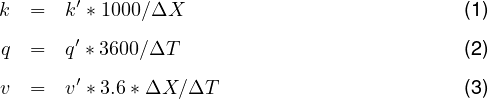
Converting between TCA and real world units seems straightforward, as we only need to suitably multiply with or divide by the temporal and spatial discretisation ΔT and ΔX, respectively. The conversions for the macroscopic traffic stream characteristics densities, flows, and space-mean speeds, as well as the microscopic vehicle speed, are as follows:
where k′,v′,q′ are the values of density, speed, flow in the units of CA, and k,q,v are the real world values of density, flow and speed.The length of our cell is 7.5 m and if our stretch of road is 1000m (i.e., 1 km ) then the no of cells in CA turns out to be 1000/7.5 =133.333 cells. So, for a single cell model if the density turns out to be “one unit” (i.e., one vehicle per cell) then in the real world its density (Kj) is 1*1000/7.5 = 133vehicles/km as per the equation. 1. The speed increment of the vehicles is the ratio of distance and time. In our case the distance is the length of one cell and time interval is one unit (sec) so the speed in km/hr is 7.5*3600/1000 =27km/hr as per the equation. 3.
In this section, we shall discuss about the Wolfram rule 184, which is used to determine the new state of the cell. In a single lane highway, rule 184 is used as a simple model for traffic flow and it forms the basis for many cellular automaton models of traffic flow.
In this model, vehicles move in a single direction, stopping and starting depending on the vehicles in front of them. The number of vehicles remains unchanged throughout the simulation. Because of this application, Rule 184 is sometimes called the “traffic rule”. Rule 184 in a simpler way can be understood as a system of particles moving both leftwards and rightwards through a one-dimensional medium. The rule set for Rule 184 is described as; At each step, if a cell with value 1 has a cell with value 0 immediately to its right, the 1 moves rightwards leaving a 0 behind. A 1 with another 1 to its right remains in place, while a 0 that does not have a 1 to its left stays a 0. This description is most apt for the application to traffic flow modeling.
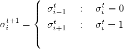
The truth table for rule 184 is shown in Table. 1. The operation of the rule is easily summarized as: “if the center cell is at state zero, shift the state of the left neighbor into the center cell, else shift the state of the right neighbor into the center cell” (equation. 4).
 | (4) |
| Si-1t | Sit | Si+1t | Sit+1 |
| 0 | 0 | 0 | 0 |
| 0 | 0 | 1 | 0 |
| 0 | 1 | 0 | 0 |
| 0 | 1 | 1 | 1 |
| 1 | 0 | 0 | 1 |
| 1 | 0 | 1 | 1 |
| 1 | 1 | 0 | 0 |
| 1 | 1 | 1 | 1 |
The first three columns are the neighborhood and the rightmost column is the state of the center cell that results from applying the transition function on the neighborhood.
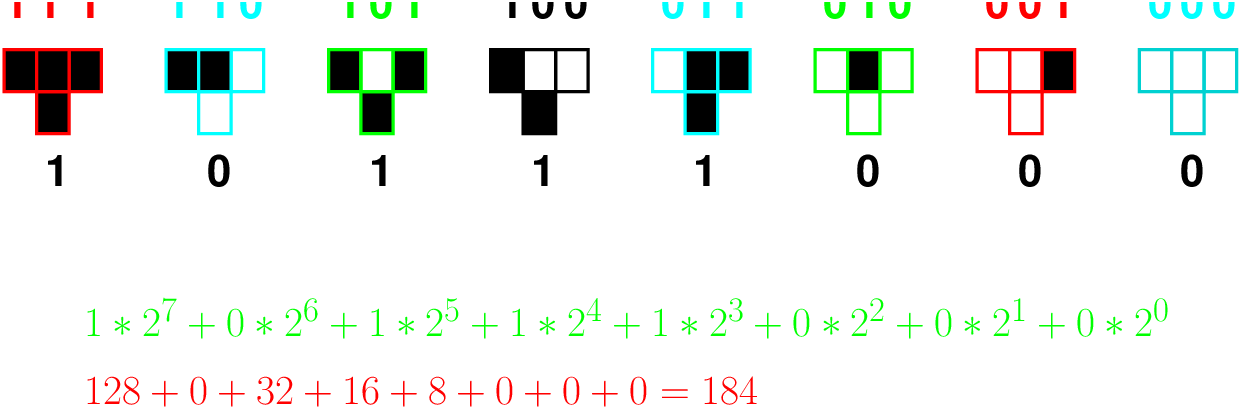
The name for this rule, Rule 184, is the Wolfram code describing the state in the Fig. 3: the bottom row of the figure, 10111000, when viewed as a binary number, is equal to the decimal number 184. All 8 possible configurations for the local neighbourhood are sorted in descending order, expressing the local transition rule (i,t) as explained by Fig. 3.
Till now we have discussed the physical and mathematical aspects of cellular automata and TCA models in particular, we shall now focus on single-cell models. As explained before each cell can either be empty, or is occupied by exactly one vehicle all vehicles have the same length li =1 cell. Traffic is also considered homogeneous, so all vehicles characteristics are assumed the same. In earlier section, 2.5 we had discussed the wolfram rule 184 which is actually a deterministic model but in the realistic traffic scenario there is stochastic term coming into picture so Wolfram rule proved to inefficient in explaining such cases and hence stochastic models are have been emerged. In the subsequent sections, we look at such stochastic TCA models (accompanied by their suggested abbreviations). In summary, Wolfram’s rule 184 (CA-184) falls under the deterministic model and the stochastic models have emerged when Nagel with the help of Schreckenberg proposed a TCA model which is the well known cellular automata in the traffic perspective.
Models that allow for the spontaneous emergence of phantom jams are called stochastic models. In 1992, Nagel and Schreckenberg proposed a TCA model that was able to reproduce several characteristics of real-life traffic flows, e.g., the spontaneous emergence of traffic jams. Their model is called the NaSch TCA, but is more commonly known as the Stochastic traffic cellular automaton (STCA).
We shall now discuss stochastic TCA models (i.e., these are probabilistic CAs) that allow for the spontaneous emergence of phantom jams. All these models explicitly incorporate a stochastic term in their equations, in order to accomplish this kind of real-life behaviour.
In 1992, Nagel and Schreckenberg proposed. A TCA model that was able to reproduce several characteristics of real-life traffic flows, e.g., the spontaneous emergence of traffic jams. Their model is called the NaSch TCA, but is more commonly known as the stochastic traffic cellular automaton (STCA). It explicitly includes a stochastic noise term in one of its rules, which we present in the same fashion as those of the previously discussed deterministic TCA models. The space is divided into cells (cell may contain vehicle or can be empty). The length of a cell is the minimum space headway available between vehicles in times of jam, and numerically it is reciprocal of jam density and is set to 7.5 m( Kj=133veh/km).
The STCA then comprises the following three rules (note that in Nagel and Schreckenberg’s original formulation, they decoupled acceleration and braking, resulting in four rules). Here we shall discuss about the NaSch model based upon its rules. There are four rules, mainly rules for acceleration, rules of deceleration, rules for randomization and lastly the vehicle updation step.
Step 1: Rule for acceleration
 | (5) |
This step reflects the general tendency of the drivers to drive as fast as possible without crossing the maximum speed limit. If the present speed is smaller than the desired maximum speed, the vehicle is accelerated. The desired speed vmax can be assumed to be distributed by a statistical distribution function where the values of vmax are only allowed to be 1, 2,..., 5 cell/Δt.
Step 2: Rule for deceleration
 | (6) |
This step ensures that the driver does’t collide with any vehicle ahead of him so that deceleration is applied to those vehicles which may collide. If the present speed is larger than the gap in the front, set v = gap. This rule avoids rear end collisions between vehicles. Note that here a very unrealistic braking rule allowing for arbitrarily large decelerations is involved. This rule forces minimum time headway of Δt s.
Step 3: Rule for randomization
 | (7) |
This step of randomization takes into account the different behavioral patterns of the individual drivers, especially, overreaction while slowing down and nondeterministic acceleration where overreaction while slowing down will be mostly responsible for the formation of traffic jams.
This rule introduces a random element into the model. This randomness models the uncertainties of driver behavior, such as acceleration noise, inability to hold a fixed distance to the vehicle ahead. Fluctuations in maximal speed, and assign different acceleration values to different vehicles. If present velocity of a vehicle is greater than zero then the velocity of the vehicle reduces by a single unit with a probability Pbrake. This rule has no theoretical background and is introduced quite heuristically.
Step 4: Vehicle updation
 | (8) |
After the above three steps the position of vehicles are updated according to their respective velocities. Even changing the precise order of the steps of the update rules stated above would change the properties of the model.
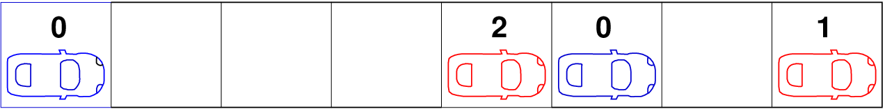
Assume a single lane stretch road divided into 8 cells and vehicles are present in the first, third, sixth, seventh cells with 2, 1, 1, 0 as their velocities respectively. Apply the rules of cellular automata.
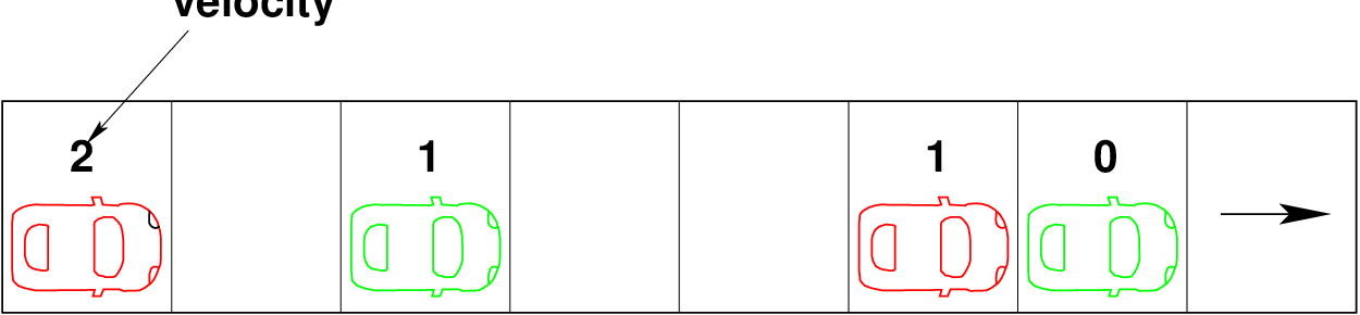
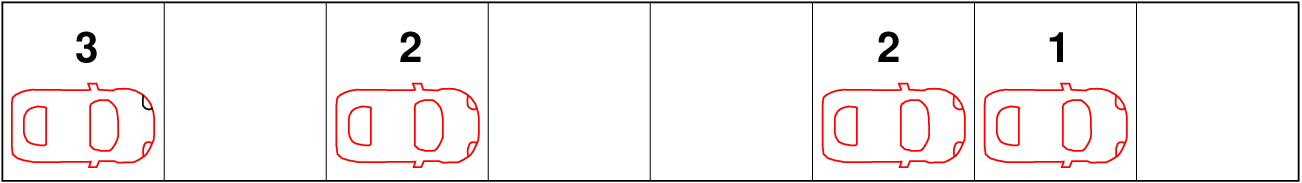
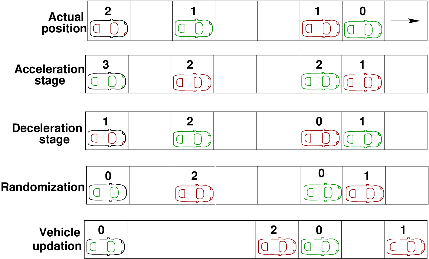
Solution Apply the CA rules (equation. 5 - 8) in a sequential way as per the requirements of acceleration, deceleration, randomization and vehicle updation. The rules are applied step wise as shown below. Step 1: Acceleration stage (according to equation. 5)

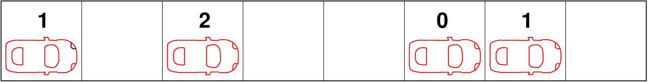
Step 2: Deceleration stage ( according to equation. 6)

Step 3: Randomization stage ( according to equation. 7)

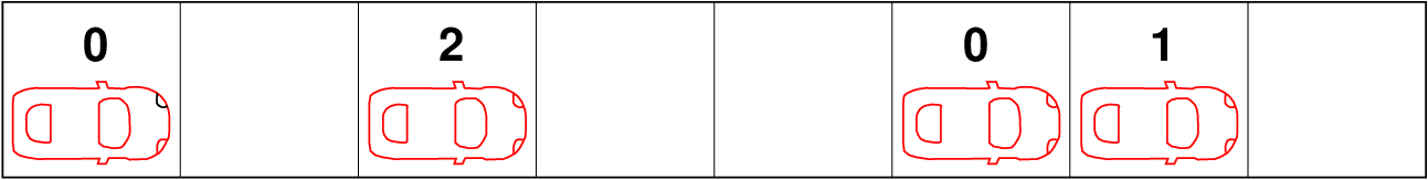
Step 4: Vehicle updation: ( according to equation. 8)

The figure below gives the reader a clear overview if all the four stages at a glance.
The concept of lane changing came into picture with the disadvantage of the single lane model of unexplained realistic traffic conditions. The reason behind this disadvantage is that a realistic traffic is usually composed of vehicle types of different desired velocities.
The presence of such vehicles will result in platooning effect. The generic two lane model is the combination of two parallel single lane models with periodic boundary conditions with some additional rules as stated in the below sections. The update step is split into two sub-steps. In first sub-step the exchange of vehicles in the two lanes, take place according to the new rule set. Vehicles are moved only sideways. They do not advance in one go. However, in reality this does not happen and this is step is also not seen. This step has a meaning when it is coordinated with the second step. In the second step, the independent single-lane updates on both lanes according to the single lane update rules.
Nagatani has formulated an oversimplified model for two-lane traffic. There are some assumptions in this model, one of which is that the maximum allowable speed of each vehicle is identical. Therefore, the model turns out to be a homogeneous type model and hence cannot explain heterogeneous traffic consisting of different types of vehicles. Some of the notations, which will be used to indicate the gaps in the lanes, are
All lane-changing rules consist of two parts: Trigger criterion (“Do I want to change the lane”) and Safety criterion (“Is it safe if I change the lane”). Once if both the criteria are fulfilled, the vehicle will change the lane.
In a two lane model proposed by Rickert, a vehicle changes its lane with a probability p, provided there is not enough gap in the current lane in front of the vehicle, if the gap in the front of the vehicle in the target lane is adequate, if it is possible without collision and finally when the lane changing activity doesn’t block someone else’s way. The above sentences are formulated in form of rules from equations. 9 to 11
 | (9) |
 | (10) |
 | (11) |
Rules 9 and 10 are called the trigger criterion and the rule 11 is called the safety criterion. These rules are applicable for both left to right and right to left lane changes and it changes the lane with probability.
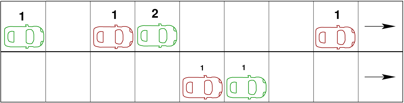
Assume a two-lane road divided into nine cells in each of its lane. In first lane vehicles are present in first (1), third (1), fourth (2), eight (1) cells and in second lane vehicles are present in fifth (1) and sixth (1) cells. The numbers in the brackets indicate the present velocities of the respective velocities. Apply the lane changing rules and determine which vehicles fulfilled the lane changing requirements.
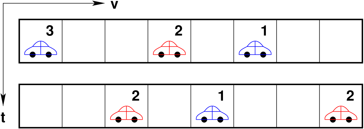
Solution Initially the solution starts with the acceleration stage of the vehicles, where the vehicles are applied with the acceleration rule (equation. 5). In the acceleration stage, a single unit increase in every vehicle, which possesses a velocity less than the maximum velocity. So stage of the vehicles after the acceleration are shown in the Fig. 5.
Lane changing is required for L1(1),L1(2),L2(1) where “L1(1)” indicates number in the subscript as its lane number and the superscript as it vehicle number in respective lanes.
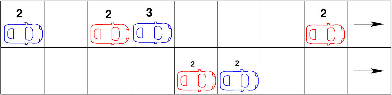
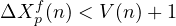
Rule 1: ΔXpp(n) < V (n) + 1 The first vehicle has a velocity two and the gap ahead of it in its current lane is 2 so according to the rule (velocity +1 > gap). Therefore, the vehicle satisfied the rule so that it can change the lane. L1(1) = (2 < 2 + 1) …satisfied. Similarly checking for all the other vehicles. L1(2) = (1 < 2 + 1) …satisfied, L2(1) = (1 < 2 + 1) …satisfied. The term gap is generally referred in two different ways, where it is explained as the distance between bumper to bumper of the vehicles. The other way to state, the term gap is the number of empty cells in front of a vehicle”. Here in the present discussion it is taken as the earlier one but anyways it depends on the reader of choosing it where a slight modification (i.e., addition of ± 1on the other side of the equations).
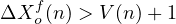
Rule 2 : (ΔXof(n) > V (n) + 1 ) (as per the rule 10) The velocity of the first vehicle is two and the gap in the target lane ahead of it is four so the rule ( gap ( target lane ) > velocity + one ) is satisfied for the first vehicle. L1(1) = (4 > 2 + 1) …satisfied. Similarly checking for other vehicles also will obtain the following results. L1(2) = (2 ⁄> 2 + 1) …rejected, and L2(1) = (34 ⁄> 2 + 1) …rejected.
Rule 3: No collision of vehicles is observed as per the pattern given.
Rule 4: (ΔXob(n) > V max ) (as per the rule 11)
The maximum velocity of any vehicle is given as four and the gap behind the first vehicle in the target lane is five which is greater than the maximum velocity so the vehicle satisfied the rule and subjected to lane change. L1(1) = (5 > 4). Therefore the first vehicle in the first lane satisfied all the four rules.
In real world traffic the vehicles don’t have unique velocities but it was an assumption in the model. So the vehicles are further divided into two types of different V max, namely V fmax, V smax, corresponding to fast vehicles and a slow vehicles. Introduction of “symmetric two lane model” for inhomogeneous traffic.
There are two types
Sequential update : This updating procedure considers each cell in the lattice one at a time. If all cells are considered consecutively, two updating directions are possible, left-to-right and right-to-left. There is also a third possibility, called random sequential update. Under this scheme and with N particles in the lattice, each time step is divided in N smaller sub steps. At each of these sub steps, a random cell (or vehicle) is chosen and the CA rules are applied to it.
Parallel update: This type of update is the classic update procedure generally used in all the models. For a parallel update, all cells in the system are updated in one and the same time step. Compared to a sequential updating procedure, this one is computationally more efficient (note that it is equivalent to a left-to-right sequential update).
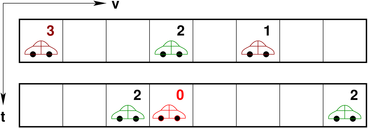
The Fig. 6 shows the updation without randomization and the Fig. 7 is with randomization where an extra deceleration is observed in second vehicle and then updation.
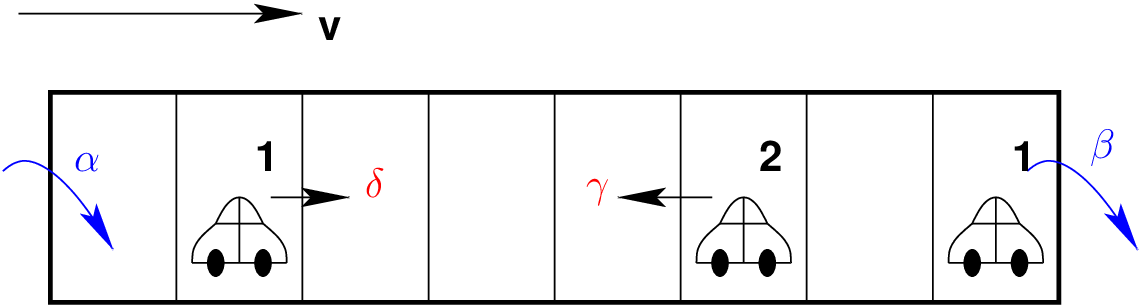
The simple exclusion process is a simplified well-known particle transport model from non-equilibrium statistical mechanics, defined on a one-dimensional lattice. In the case of open boundary conditions (i.e., the bottleneck scenario), particles enter the system from the left side at an entry rate α , move through the lattice, and leave it at an exit rate β. The term ‘simple exclusion’ refers to the fact that a cell in the lattice can only be empty, or occupied by one particle.
When moving through the lattice, particles move one cell to the left with probability, and one cell to the right with probability γ. When γ = δ, the process is called the symmetric simple exclusion process (SSEP); if γ = δ then it is called the asymmetric simple exclusion process (ASEP). Finally, if we set γ = 0 and δ = 1, the system is called the totally asymmetric simple exclusion process (TASEP). If we consider the TASEP as a TCA model, then all vehicles move with V max = 1 cell/time step to their direct right-neighbouring cell, on the condition that this cell is empty. The process is shown in the below Fig. 8.
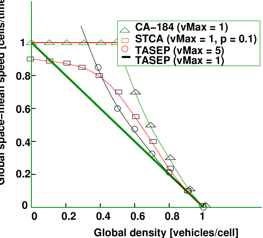
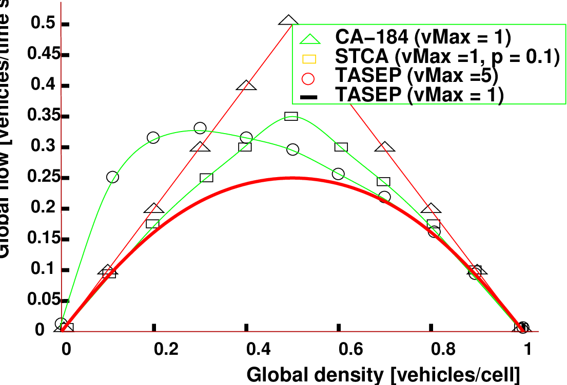
The above Fig. 9 gives a differentiation between four types of models and interestingly it is observed that the TASEP with V max = 1 has a trend of the Greenshield model and following a linearity in the speed-density relation. The same trend is also observed in the below Fig. 10 flow density curve.
I wish to thank several of my students and staff of NPTEL for their contribution in this lecture.
I wish to thank my student Mr. Manikanta Kumar for his assistance in developing the lecture note, and my staff Ms. Reeba in typesetting the materials. I also wish to thank several of my students and staff of NPTEL for their contribution in this lecture. I also appreciate your constructive feedback which may be sent to tvm@civil.iitb.ac.in
Prof. Tom V. Mathew
Department of Civil Engineering
Indian Institute of Technology Bombay, India
_________________________________________________________________________
Thursday 31 August 2023 01:04:23 AM IST