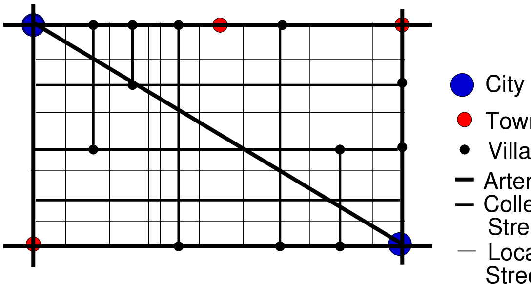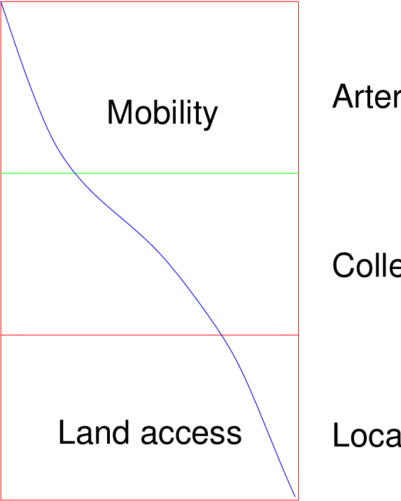
Figure 1: Relationship of functionally classified systems in service traffic mobility and
land access
Cities and traffic have developed hand-in-hand since the earliest large human settlements and forcing inhabitants to congregate in large urban areas and in turn enforcing need of urban transportation. To develop efficient street transportation, to serve effectively various land use in an urban area, and ensure community development, it is desirable to establish a network of streets divided into systems, each system serving a particular function or particular purpose. Accordingly, a community should develop an ultimate street-classification in which each system has a specific transportation service function to perform. There are several operational performance measures and level of services (LOS) which have to be taken into account to evaluate the system of streets. Increasing population of urban areas due to shifting of people from rural to urban areas and thus certainly increasing vehicular population on urban streets, have caused problems of congestion in urban areas. Road traffic congestion poses a challenge for all large and growing urban areas. This document provides a summary of urban street with respect to their classification, related operational performance measures and level of services (LOS) involved in each class of urban street and it also provides strategies necessary for any effective congestion management policy to curb the congestion.
There are three ways of classifying urban streets
Functional classification is the process by which streets and highways are grouped into classes, or systems, according to the character of service they are intended to provide. Basic to this process is the recognition that individual roads and streets do not serve travel independently in any major way. Rather, most travel involves movement through a network of roads. It becomes necessary then to determine how this travel can be channelized within the network in a logical and efficient manner. Functional classification defines the nature of this channelization process by defining the part that any particular road or street should play in serving the flow of trips through a highway network. The four functional systems for urbanized areas are:
General idea of various streets as per their mobility and land use is shown in the Fig. 1.
Arterial streets are basically meant to carry longer and through traffic. Function of arterial is to provide access to commercial and residential land uses. A downtown street not only carries through traffic but also turning traffics and it resembles arterials. As shown in Fig. ?? mobility of principal arterials is high but land access is very low. Major arterial serves as principal network for through traffic flow. This should be connected with principal traffic generations, important rural highways entering the city. It should be well coordinated with existing and proposed expressway system for good distribution and circulation of through traffic and continuity of routes should be maintained. In every urban environment there exists a system of streets and highways which can be identified as unusually significant to the area in which it lies in terms of the nature and composition of travel it serves. In smaller urban areas (population under 50,000) these facilities may be very limited in number and extent and their importance may be primarily derived from the service provided to travel passing through the area. In larger urban areas their importance also derives from service to rural oriented traffic, but equally or even more important, from service for major movements within these urbanized areas. The principal arterial system should carry the major portion of trips entering and leaving the urban area, as well as the majority of through movements desiring to bypass the central city. In addition, significant intra-area travels, such as between central business districts and outlying residential areas between major inner city communities or between major suburban centers should be served by this system. Frequently the principal arterial system will carry important intra urban as well as intercity bus routes. Finally, this system in small urban and urbanized areas should provide continuity for all rural arterials which intercept the urban boundary.
The minor arterial street system should interconnect with and augment the urban principal arterial system and provide service to trips of moderate length at a somewhat lower level of travel mobility than principal arterials. This system also distributes travel to geographic areas smaller than those identified with the higher system. The minor arterial street system includes all arterials not classified as a principal and contains facilities that place more emphasis on land access than the higher system, and offer a lower level of traffic mobility. Such facilities may carry local bus routes and provide intra-community continuity, but ideally should not penetrate identifiable neighborhoods. This system should include urban connections to rural collector roads where such connections have not been classified as urban principal arterials. The spacing of minor arterial streets may vary from half to one km in the central business district to 4 to 5 km in the suburban fringes, but should normally be not more than 2 km in fully developed areas.
This system of streets includes all distributer and collector streets. Function of this system is serving between major arterials and local streets to connect adjacent neighborhood areas placed approximately at half miles intervals to accommodate local through traffic movements and interconnect local streets with the major arterial street system. Unlike arterials their operation is not always dominated by traffic signals.
Local streets are primarily meant for direct access to residential commercial, industrial or other abutting property. All through traffics should be discouraged on local streets. Land access is very high but mobility is very low for local streets.
This classification basically depends upon speed limits, signal density, driveways / access point density etc.
These are the streets with very low driveway or access point density. These are provided with separate right turn lanes and; no parking is permitted on street. Streets may be multilane divided or undivided or two lane facility with shoulders. Signals are infrequent and spaced at long distances. Road side development is very low. A speed limit on these roads is 75 to 90 kmph.
They represent streets with a low driveway/access-point density,separate or continuous right turn lane and some portions where parking is permitted. These roads possess comparatively higher density of roadside development than that on high speed streets. It has about three signals per Km. and speed limit on these roads is 65 to 75 kmph.
They represent urban streets with moderate driveway/access point density. Like sub-urban streets they also have some separate or continuous right turn lane and some portions where parking is permitted. These roads possess comparatively higher roadside development than that on sub-urban streets. It has about two to six signals per Km. and speed limit on these roads is 50 to 60 Kmph.
They represent urban streets with high driveway/access point density. These are usually provided with road side parking. It has highest road side development density among all above stated four classes. Signal density is about four to eight per Km. Speed limit is 40 to 55 Kmph.
This type of classification considers for combination of functional and design classes divided into four classes viz. I, II, III, IV which reflects a unique combination for of street function and Design, as shown in table 1 and related signal densities are shown in table 2.
| Design category | Functional category
| |
| Principal arterial | Minor arterial | |
| High speed | I | NA |
| Suburban | II | II |
| Intermediate | II | III or IV |
| Urban | III or IV | IV |
| Urban Street Class | Signal density | Free flow |
| (signals/km) | speed(kmph) | |
| I | 0.2 | 80 |
| II | 2 | 65 |
| III | 4 | 55 |
| IV | 6 | 45 |
Engineer has to quantify how well the ’system’ or ’facility is working’. The facilities will usually assembled by specific qualitative and quantitative index of flow characteristics termed as Level of Service (LOS), in this regard engineer has to do following works.
As far as operational performance of urban streets is considered we are interested in determining arterial level of service which is discussed in succeeding section.
Urban streets LOS is mainly based on average travel speed for the segment or for the entire street under consideration. The average travel speed is computed from the running times on the urban street and the control delay of through movements at signalized intersections. The control delay is the portion of the total delay for a vehicle approaching and entering a signalized intersection. Control delay includes the delays of initial deceleration, move-up time in the queue, stops, and re-acceleration, these delays are also known as intersection approach delays.
The LOS for urban streets is influenced both by the number of signals per kilometer and by the intersection control delay. Inappropriate signal timing, poor progression, and increasing traffic flow can degrade the LOS substantially. Streets with medium-to-high signal densities (i.e., more than one signal per kilometer) are more susceptible to these factors, and poor LOS might be observed even before significant problems occur. On the other hand, longer urban street segments comprising heavily loaded intersections can provide reasonably good LOS, although an individual signalized intersection might be operating at a lower level. The term through vehicle refers to all vehicles passing directly through a street segment and not turning. Considering all the above aspects, HCM provides a seven step methodology to determine the level of service of an arterial which will be discussed in following section.
HCM method of arterial performance measurement involves seven steps which aim to compute ’average travel speed’ of arterial to measure the Level of Service. These seven steps are as follows,
The above flow chart shows the steps to determine LOS in a schematic form. Further in this section we are going to discuss these seven steps in detail.
Establishing the arterial is the very first step in the process of determining the LOS. In this step, an engineer has to define arterial segment or entire arterial whose LOS is to be determined. Arterial may be established by arterial class, its flow characteristics and signal density. Arterial class may be defined as per its free flow speed as explained in step 2 as follows.
Free flow speed is the speed on the arterial which most of the drivers choose if they had green indication and they are alone in the direction of movement are not the part of platoon) but have to be conscious about all other prevailing conditions. (e.g. Block spacing, contiguous land use, right of way, characteristic, pedestrian activity, parking, etc.) Free flow speed should be measured at just the time when the entire factors are present except for the prevailing traffic levels and red indication. An arterial can be classified on the basis of its free flow speed as explained under the section design based classification and combined classification . The following table 3 can be used to determine the arterial class.
| Free flow | ||||
| speed (kmph) | I | II | III | IV |
| Speed range | 90 to 70 | 70 to 55 | 55 to 50 | 55 to 40 |
| Typical value | 80 | 65 | 55 | 45 |
After determining the arterial class it is required to be more specific about the particular section of an arterial for which LOS is to be determined. The arterial section may be mid block or intersection. Generally signalized intersection is taken into account to determine intersection approach delays which are further required to determine level of service.
There are two principal components for the total time that a vehicle spends on a segment of an urban street. These are running time and control delay at signalized intersections. To compute the running time for a segment, the analyst must know the street’s classification, its segment length, and it’s free flow speed. Arterial running time can be obtained by Travel time studies, information of running times from local data and intersection delays etc.
Intersection approach delay is the correct delay which is to be used in arterial evaluation. It gives consideration not only for absolute stopped delay but also for the delay in retarding the vehicle approaching at signal for stopping and re-accelerating on starting of green. It is longer than the stopped delay. This can be related to intersection stopped delay and is computed by,
 | (1) |
where, D = intersection approach delay (sec/veh), and d = intersection stopped delay (sec/veh). Delay at intersection approach is of special interest because it is a Measure of Effectiveness (MOE) used to quantify LOS. To determine intersection approach (or control) delay it is necessary to calculate stopped delay which is discussed below.
Stopped vehicles on intersection are counted for intervals of 10 to 20 seconds. It is assumed that vehicles counted as ’stopped’ during one of these intervals will be stopped for the length of the interval. Measuring the stopped delays involves following steps.
In an intersection the following data was observed for stopping times for vehicles as tabulated in table 4. Calculate intersection approach delay for the given data set. Total exiting vehicles: 100.
| Minute | 0 sec | 15 sec | 30 sec | 45 sec |
| 5.00 pm | 2 | 4 | 1 | 3 |
| 5.01 pm | 4 | 5 | 3 | 0 |
| 5.02 pm | 6 | 3 | 2 | 1 |
| 5.03 pm | 2 | 5 | 4 | 3 |
| 5.04 pm | 4 | 2 | 6 | 4 |
| 5.05 pm | 5 | 4 | 1 | 1 |
| 5.06 pm | 1 | 2 | 5 | 5 |
| 5.07 pm | 4 | 3 | 3 | 3 |
| 5.08 pm | 2 | 5 | 2 | 2 |
| 5.09 pm | 3 | 1 | 4 | 2 |
| Total | 33 | 34 | 31 | 24 |
Solution: Total of stopped-vehicle counts (density counts) for study sample is: 33+34+31+24=122 veh. Each of the vehicle interval is 15 seconds. Aggregate delay for the 10 minutes study period is, 122× 15 sec=1830 veh-sec. Average stopped delay per vehicle for study period of 10 minutes is, 1830/100 =18.3 sec per vehicle. That is, d=18.3 sec per vehicle. We use this in the first equation. So, intersection approach (or control) delay D
 |
Arterial LOS is based on the ’average travel speed’ for segment, section or entire arterial under consideration. Arterial average travel speed is given by
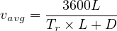 | (2) |
where, vavg = arterial or segmental average travel speed (Kmph), L = arterial or segmental length (Km), Tr = total of the running time per kilometer on all segments in the arterial or section (seconds), D = total of the approach delay at all intersections within the defined arterial (seconds). It is the actual speed in consideration with the additional effect of control and all stop delays. It is the measure by which LOS is defined.
This is the last step of determination of LOS. After calculation of average travel speed we can determine the level of service of an arterial by using Table 5.
| LOS | ||||
| I | II | III | IV | |
| A | > 72 | > 59 | > 50 | > 41 |
| B | > 56 | > 46 | > 39 | > 32 |
| C | > 40 | > 33 | > 28 | > 23 |
| D | > 32 | > 26 | > 22 | > 18 |
| E | > 26 | > 21 | > 17 | > 14 |
| F | > 26 | < 21 | < 17 | < 14 |
Consider an arterial which has free flow speed of 65 kmph and average running time of
vehicles is 145 sec/km determine LOS for this arterial.
Solution: From Table 5 we can find LOS of an arterial. As free flow speed is 65 kmph by using table 3 we can classify this as Arterial Class II, Now we should know average travel speed, to find out LOS. Delay is determined in problem 1. Hence D=23.79sec/veh.
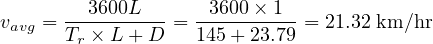 |
As average travel speed is 21.32 kmph we can have LOS as ’E’ from Table 5.
When demand on a facility exceeds the capacity Congestion takes place. The travel time or delay is in excess of that normally incurred under light or free flow traffic condition. The travel time or delay is in excess of agreed upon norm which may vary by type of transport facility, travel mode, geographical location, and time of day. In the procedure for congestion management initially we have to find out the root cause of congestion and finding out the remedies for managing the congestion, updating the signalization if it is needed. It is always better to use good signalization for minimizing impact of congestion. We can provide more space by making use of ’turn bays’ if geometry permits. Parking restrictions also help in congestion management on urban streets. Now we will discuss some important strategies to manage the congestion on urban streets.
Basically at street level congestion can be encountered by following ways,
Signal based remedies for congestion management can be achieved by implementing following two strategies,
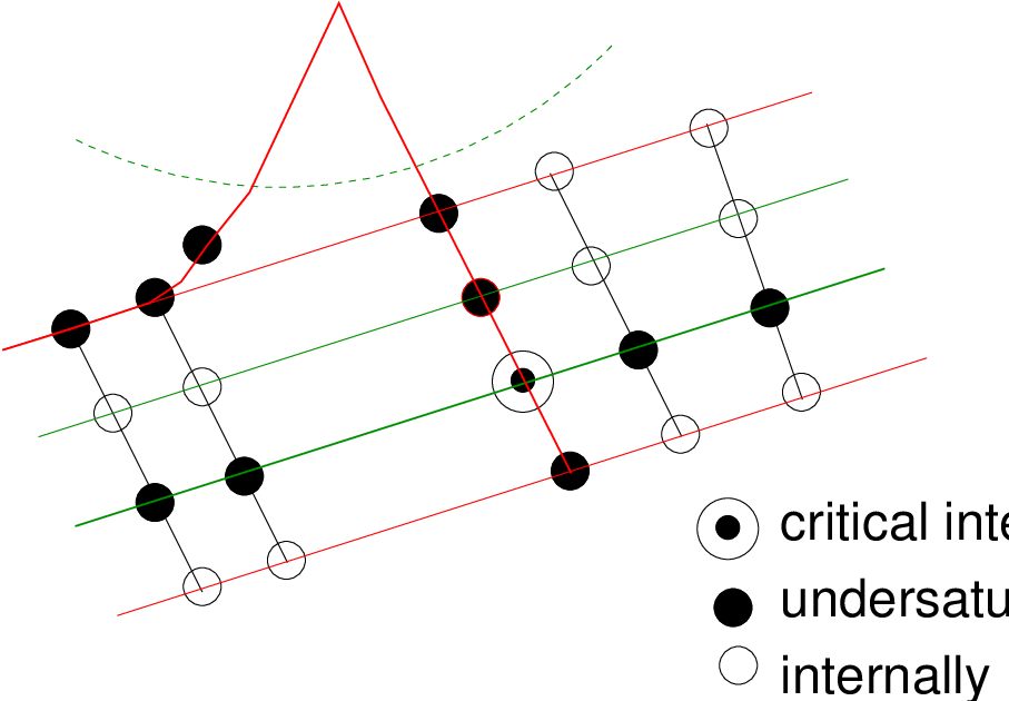
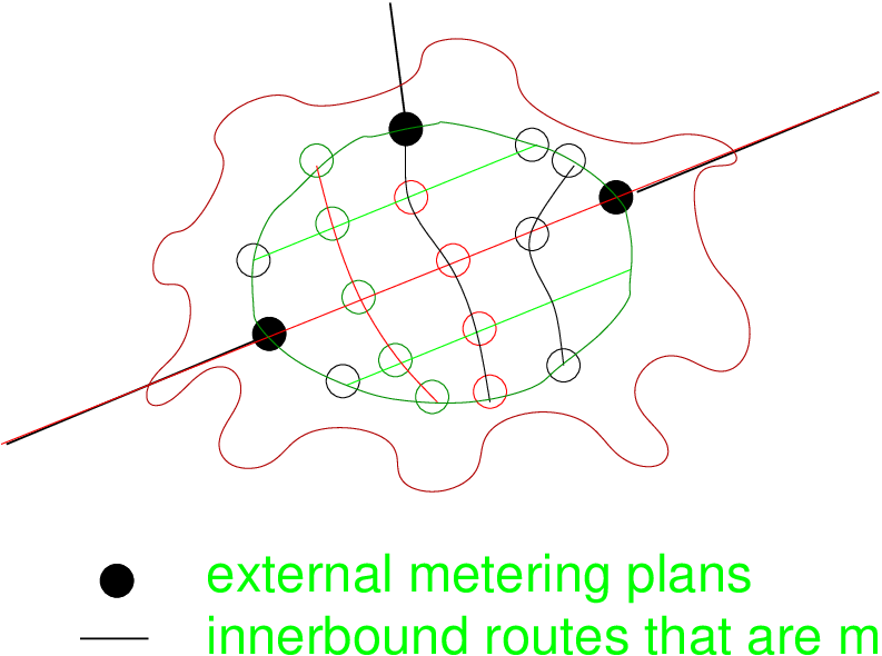
It is the congestion management policy for street congestion to limit the volumes arriving at critical locations. It uses some control strategies within the congestion networks by storing vehicles at links defined to be part of system under control. It should be noted that metering concept does not explicitly minimize delays and stops but manages queue formation. There are three types of metering strategies,
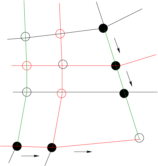
It deals with upstream control by creating moving storage situation on upstream link. It manages congestion by limiting turn-in flows from cross streets and preserving arterials for their through flow by metering from face of back up from outside as shown in Fig. 6
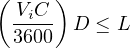
If on any intersection higher cycle time is provided then it will certainly create problems like increase in queue length and platoon length discharged and it will lead to increase in blockage of intersection, with substantial adverse impact on system capacity. This is particularly when short link lengths are involved. Length of downstream space should be greater than queue length to store the vehicles. Note that a critical lane flow of Vi nominally discharges Vi*C/3600 vehicles in a cycle. If each vehicle requires D meters of storage space, the downstream link would be
 | (3) |
where,  = no. of vehicles per cycle, D= storage space required for each vehicle, L=
available downstream space in m. (This may be set by some lower value to keep the queue
away from the discharging intersection, or to allow for turn-ins.) Equation may be re-arranged
as,
= no. of vehicles per cycle, D= storage space required for each vehicle, L=
available downstream space in m. (This may be set by some lower value to keep the queue
away from the discharging intersection, or to allow for turn-ins.) Equation may be re-arranged
as,
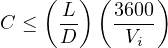 | (4) |
Note that V i in this case is the discharge volume per downstream lane, which may differ from the demand volume, particularly at the fringes of the system being considered. Note that only rather high flows (maximum f > 800 veh per hour per lane (vphpl)) and short blocks will create very severe limits on the cycle length. However, these are just the situations of at most interest for extreme congestion situations. An illustrative example to show the requirement of shorter cycle length is given below.
Flow on an critical lane is 300 veh/h, cycle time is 80 seconds, suppose storage space required per lane vehicle is 6m as an average and space available on downstream is 30 m, find whether the space is sufficient and comment on the result and suggest some remedy if required.
Solution:
Given: V i = 300 veh/h, C = 80 sec, and L = 30 m. Vehicles discharged by a critical lane
per cycle to be found out and which is given by, ( ) = 300 * 80/3600 = 60/9 =6.6 veh/cycle.
Therefore, space required for storing these vehicles for cycle time is, = 6.6 * D, = 6.6 * 6, =
39.6 m. ≈ 40 m. So, 40 m > 30 m (length of downstream storage i.e. space available), So
length is inadequate. As the length is fixed the only possible variable is ’cycle time’ so
we will reduce the cycle time, let the new cycle time be, 40 seconds instead of 80
seconds. Space required will be get reduced to half i.e. 20m which is lesser than the
available space i.e. 30m so it is feasible to reduce the cycle length to manage the
congestion.
) = 300 * 80/3600 = 60/9 =6.6 veh/cycle.
Therefore, space required for storing these vehicles for cycle time is, = 6.6 * D, = 6.6 * 6, =
39.6 m. ≈ 40 m. So, 40 m > 30 m (length of downstream storage i.e. space available), So
length is inadequate. As the length is fixed the only possible variable is ’cycle time’ so
we will reduce the cycle time, let the new cycle time be, 40 seconds instead of 80
seconds. Space required will be get reduced to half i.e. 20m which is lesser than the
available space i.e. 30m so it is feasible to reduce the cycle length to manage the
congestion.
If the problem of congestion does not get resolved by signalization the next set of actions are summarized in two words more space means there is need of provision of additional lanes or some other facility. It can be achieved by adding left turn bays / right turn bays, removing obstructions to through flows by adding more space and free movements Some non-signal based remedies are given below,
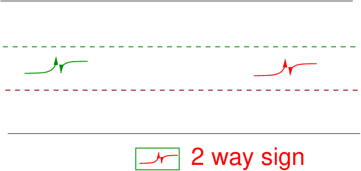
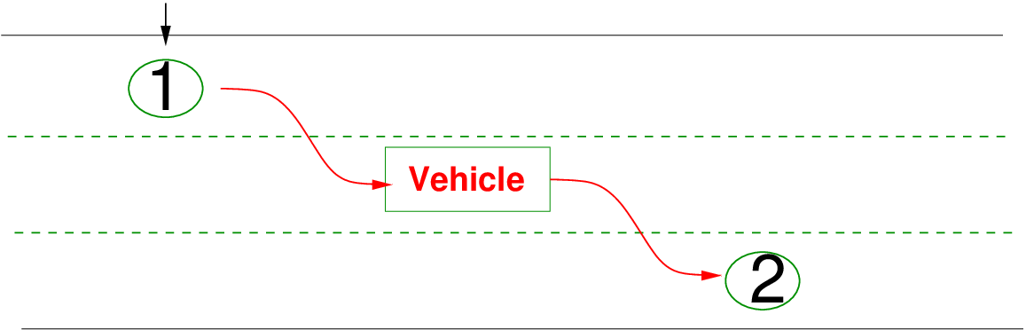
On suburban and urban arterials dedication of a central lanes shown in Fig. 8 for turns in either direction is provided. This also allows for storage and vehicles to make their maneuvers in two distinct steps.
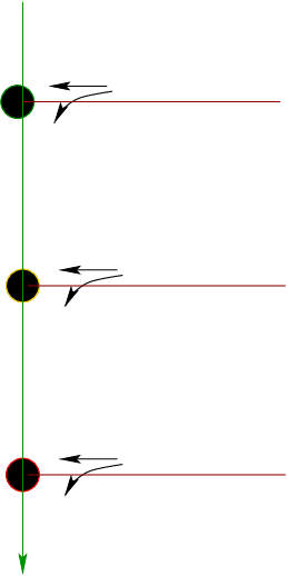
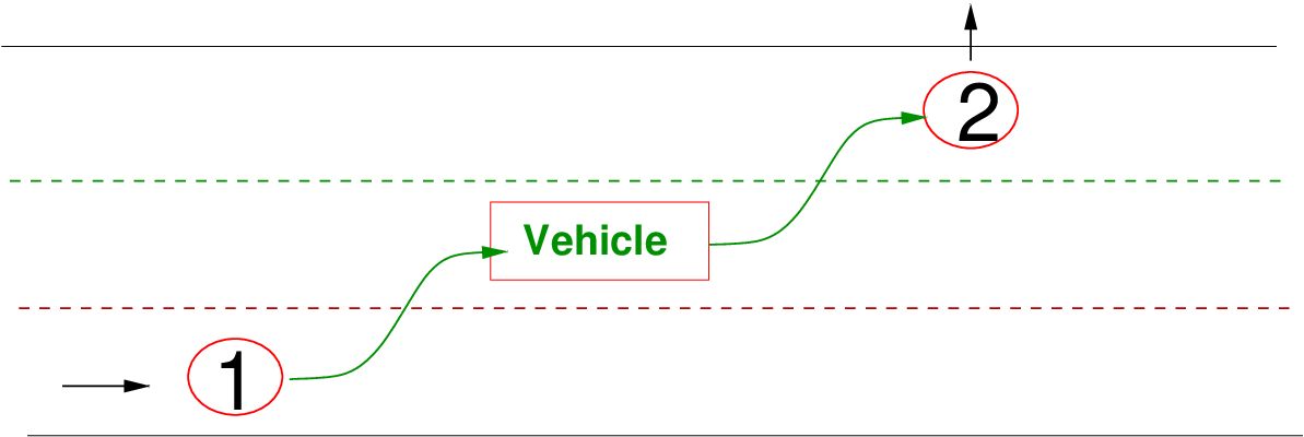
Leaving the arterial and entering it is separated into two distinct steps. Vehicles leaving (Fig. 9) the arterial do not have to block a moving lane while waiting for a gap in the opposing flow. Entering vehicles (Fig. 10) do not have to wait for a gap simultaneously in both directions. The Figure 8 shown above is the road sign for two way left turn lane which indicates that the center lane is provided exclusively for two way left turning traffic.
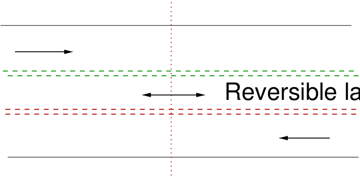
Reversible lanes shown in Figure 8 have great advantage of matching lane availability to the peak demand. Lanes are reversible means can be split into various combinations for different times of day to match the demand.
E.g. eight lanes can be split into 6:2 or 5:3 and so forth if required to match up for the demand. It should be noted that some jurisdictions have combined two-way lanes and reversible lanes on same arterial ’because combination of peak-period congestion and increased road side development’. The concerns with reversible lanes and relates to the misuse and lanes by the driver (particularly the unfamiliar driver), despite the signalization over the lanes.
High occupancy vehicle (HOV) lanes are designed to help move more people through congested areas. HOV lanes offer users a faster, more reliable commute, while also easing congestion in regular lanes - by moving more people in fewer vehicles. HOV lanes on provincial highways are reserved for any of the following passenger vehicles carrying at least two people (often referred to as 2+):
In addition, vehicles with a special green licence plate (plug-in hybrid electric or battery electric vehicle) A bus of any type can use an HOV lane, even without passengers. This helps buses keep to their schedules and provide reliable, efficient service. Emergency vehicles are permitted to use the HOV lanes at all times.
Congestion can be managed by prohibiting the kerb parking. Kerb parking means on street parallel parking. If such parking is avoided it implies oblique and right angled parking is also prohibited and hence provides more space for traffic flow so congestion is minimized.
Longitudinal lane markings such solid white lines and broken white lines restricts overtaking maneuver of vehicles which encourages mix through traffic flow unobstructed resulting in reducing the congestion.
This topic can be read in reference to congestion management by signal based remedies. Offset on an arterial are usually set to move vehicles smoothly along the arterial, as is logical. Equity offset allows the congested arterial to have its green at upstream intersection until the vehicle just begin to move , then switch the signal, so that these vehicles flush out the intersection, but no new vehicles continue to enter.
This topic can be referred under signal based congestion management remedies. It is the procedure of allocating the ’available green’ in proportion to the relative demands. It is sometimes desirable to split green as per demand of various routes to meet peak hour demands of respective routes.
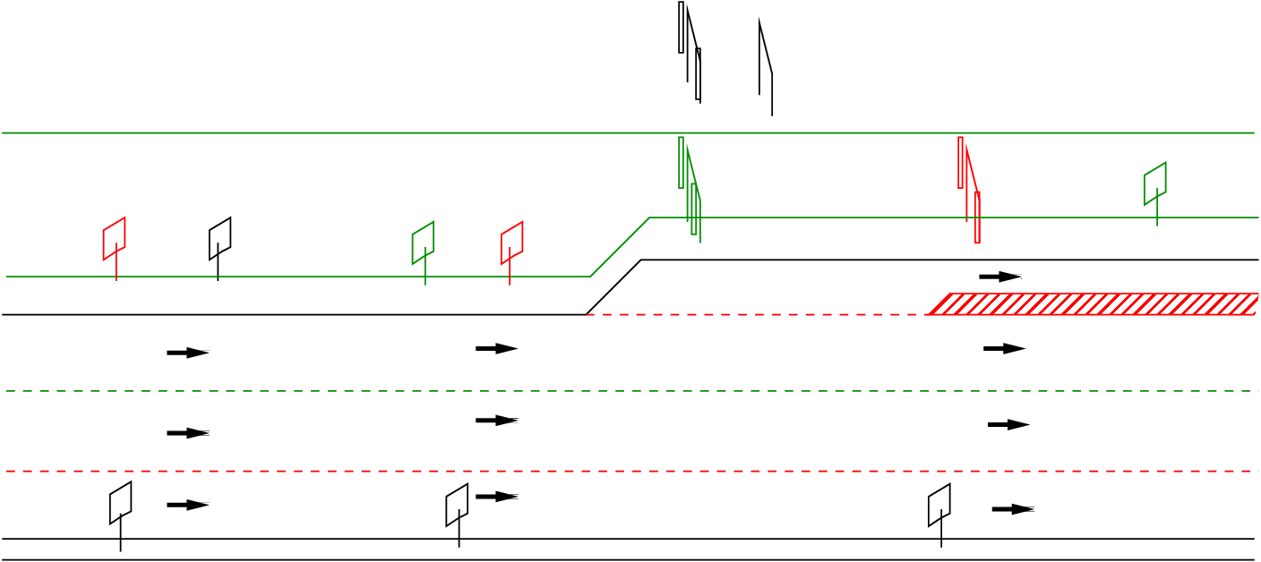
This topic can be referred as non signal based remedies On provincial highways HOV lanes are developed by adding a new inside (leftmost) lane to existing corridors. Where the HOV lane begins, signs on the left side of the highway inform carpools and buses to move left into the new lane. An overhead sign indicates the beginning of the HOV lane. In some locations, where a highway on-ramp used to end, the on-ramp lane has been extended as the new HOV lane. In this situation, motorists not permitted to use the HOV lane have to exit that lane before the start of the HOV lane designation. Overhead signs at 1 kilometre and again at 500 metres before the start of the HOV lane designation advise drivers to exit the lane. Overhead signing and closely spaced white broken lines and diamond symbol pavement markings indicate the beginning of the HOV lane (Figure 12).
It can be understood that urban streets are integral part of transportation system. Urban streets plays vital role in development of country. These are classified on their function, design for various considerations taking into account. Performance measures are to be worked out to determine LOS. Congestion is a huge problem which can be curbed by some preventive measures and design strategies. Signalized remedies are more efficient than any other measures of street congestion management. Non signalized remedies can be used to manage congestion by providing more space in terms of extra lanes.
I wish to thank several of my students and staff of NPTEL for their contribution in this lecture. I wish to thank specially my student Mr. Rohit R. Ghodke for his assistance in developing the lecture note, and my staff Mr. Rayan in typesetting the materials. I also appreciate your constructive feedback which may be sent to tvm@civil.iitb.ac.in
Prof. Tom V. Mathew
Department of Civil Engineering
Indian Institute of Technology Bombay, India
_________________________________________________________________________
Wednesday 27 September 2023 10:44:06 PM IST