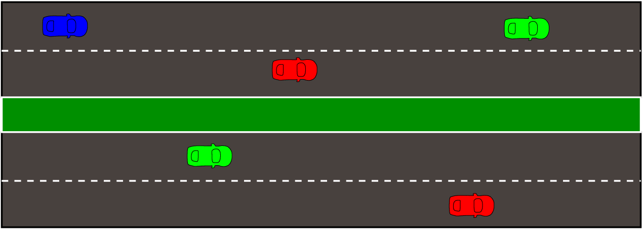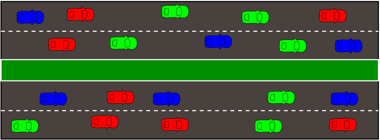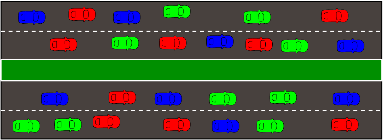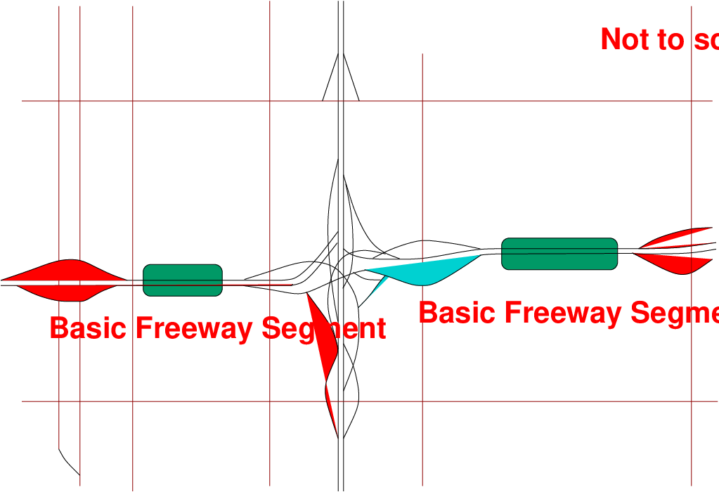
Figure 1: Basic freeway segment
A freeway is defined as a divided highway with full control of access and two lanes for the exclusive use of traffic in each direction. Freeways were originally intended to serve longer trips of generally regional and interurban character. Traffic on freeways differs from that on city streets and rural roads in that it moves at higher speeds (depending on traffic conditions, design standards, etc.), more smoothly, and at much larger rates of flow. Speed limits are generally higher on freeways, and are occasionally non-existent. Because higher speeds reduce decision time, freeways are usually equipped with a larger number of guide signs than other roads, and the signs themselves are physically larger. Guide signs are often mounted on overpasses or overhead gantries so that drivers can see where each lane goes. Access to freeways is typically provided only at grade-separated interchanges, though lower-standard right-in/right-out access can be used for direct connections to side roads. This chapter basically describes the capacity and level of service. Later weaving phenomenon in has been described.
Freeway provides uninterrupted traffic flow on a freeway. Traffic on freeway is free-flowing. All cross-traffic (and left-turning traffic) is relegated to overpasses or underpasses, so that there are no traffic conflicts on the main line of the highway which must be regulated by traffic lights, stop signs, or other traffic control devices. Specific features are:
A freeway is composed of following three components
Basic freeway are that part of segment of freeway which are outside of the influence area of ramps or weaving areas of freeway.
We can see in Fig.1 that a basic freeway segment is independent of the ramps and weaving areas and the flow in such section occurs smoothly at the much larger rates. Merging and diverging of traffic occurs where on-or-off ramps join the basic freeway segment. Weaving occurs when vehicles cross each other’s path while travelling on freeway lanes. The exact point at which basic freeway segment begins or ends- that is, where the influence of weaving areas and ramp junctions has dissipated- depends on local conditions, particularly the level of service operating at the time. If traffic flow is light, the influence may be negligible, whereas under congested conditions, queues may be extensive.
The base conditions under which the full capacity of a basic freeway segment is achieved are good weather, good visibility, and no incidents or accidents. For the analysis procedures in this chapter, these base conditions are assumed to exist. A set of base conditions for basic freeway segments has been established. These conditions serve as a starting point for the
Base conditions for intersection approaches include the following:
Freeway capacity is defined as:
the maximum sustained 15-min flow rate, expressed in passenger cars per hour per lane, that can be accommodated by a uniform freeway segment under prevailing traffic and roadway conditions in one direction of flow.
Capacity analysis is based on freeway segments with uniform traffic and roadway conditions. If any of the prevailing conditions change significantly, the capacity of the segment and its operating conditions change as well. Therefore, each uniform segment should be analysed separately.
Roadway conditions include geometric and other elements. In some cases, these influence the capacity of a road; in others, they can affect a performance measure such as speed, but not the capacity or maximum flow rate of the facility. Roadway factors include the following:
Traffic conditions that influence capacities and service levels include vehicle type and lane or directional distribution.
Vehicle type The entry of heavy vehicles - that is, vehicles other than passenger cars (a category that includes small trucks and vans) - into the traffic stream affects the number of vehicles that can be served. Heavy vehicles are vehicles that have more than four tires touching the pavement. Trucks, buses, and recreational vehicles (RVs) are the three groups of heavy vehicles.
Directional and Lane Distribution In addition to the distribution of vehicle types, two other traffic characteristics affect capacity and level of service: directional distribution and lane distribution. Each direction of the facility usually is designed to accommodate the peak flow rate in the peak direction. Typically, morning peak traffic occurs in one direction and evening peak traffic occurs in the opposite direction. Lane distribution also is a factor on multi lane facilities. Typically, the shoulder lane carries less traffic than other lanes.
For interrupted-flow facilities, the control of the time for movement of specific traffic flows is critical to capacity and level of service. The most critical type of control is the traffic signal. The type of control in use, signal phasing, allocation of green time, cycle length, and the relationship with adjacent control measures affect operations. Stop signs and yield signs also affect capacity, but in a less deterministic way. A Impact of control conditions traffic signal designates times when each movement is permitted; however, a stop sign at a two-way stop-controlled intersection only designates the right-of-way to the major street. The capacity of minor approaches depends on traffic conditions on the major street. An all-way stop control forces drivers to stop and enter the intersection in rotation. Capacity and operational characteristics can vary widely, depending on the traffic demands on the various approaches.
Level of service is defined as:
qualitatively measures both the operating conditions within a traffic system and how these conditions are perceived by drivers and passengers.
These operational conditions within a traffic stream are generally described in terms of service measures as speed and travel time, freedom to maneuver, traffic interruptions, and comfort and convenience. The three measures of speed, density and flow are interrelated. If values of two are known, the third can be computed. Six LOS are defined for each type of facility that has analysis procedures available. Letters designate each level, from A to F, with LOS A representing the best operating conditions and LOS F the worst. Each level of service represents a range of operating conditions and the driver’s perception of those conditions. Safety is not included in the measures that establish service levels.
In all cases, breakdown occurs when the ratio of existing demand to actual capacity forecast demand to estimated capacity exceeds 1.00. The figures 2-7 given below gives a better idea of the LOS classification done on the basis of density of the traffic stream.
A basic freeway segment can be characterized by three performance measures: density in
terms of passenger cars per kilometer per lane, speed in terms of mean passenger-car
speed, and volume-to-capacity (v/c) ratio. Each of these measures is an indication of how well
traffic flow is being accommodated by the freeway. The measure used to provide an estimate
of level of service is density. The three measures of speed, density, and flow or volume are
interrelated. If values for two of these measures are known, the third can be computed.
Level of service of an existing freeway is determined considering it as a stretch of basic freeway segment. It means that we have to take all the base conditions decided for basic freeway segment as a standard or initial input. The following steps are followed to determine the level of service of a freeway.
The steps involved in calculation of LOS are-
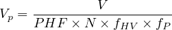
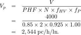
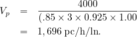
The hourly flow rate must reflect the influence of heavy vehicles, the temporal variation of traffic flow over an hour, and the characteristics of the driver population. These effects are reflected by adjusting hourly volumes or estimates, typically reported in vehicles per hour (veh/h), to arrive at an equivalent passenger-car flow rate in passenger cars per hour (pc/h). The equivalent passenger-car flow rate is calculated using the heavy-vehicle and peak-hour adjustment factors and is reported on a per lane basis (pc/h/ln). The flow rate can be given as-
 | (1) |
where, V = hourly volume, PHF = peak hour factor (0.80-0.95), N = no. of lanes, fHV = heavy vehicle adjustment factor, fP = driver population factor
Peak hour factor (PHF) The peak-hour factor (PHF) represents the variation in traffic flow within an hour. Observations of traffic flow consistently indicate that the flow rates found in the peak 15-min period within an hour are not sustained throughout the entire hour.
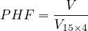 | (2) |
Where, V = hourly volume in veh/hr for hour of analysis, V 15 = Maximum 15-min flow rate
within peak hour, 4 = number of 15-min period per hour.
On freeways, typical PHFs range from 0.80 to 0.95. Lower PHFs are characteristic of rural
freeways or off-peak conditions. Higher factors are typical of urban and suburban peak-hour
conditions. Field data should be used, if possible, to develop PHFs representative of local
conditions.
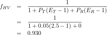
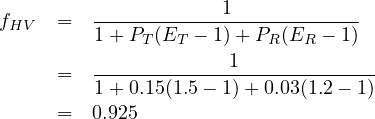
Heavy vehicle adjustment factor (fHV ) Freeway traffic volumes that include a mix of vehicle types must be adjusted to an equivalent flow rate expressed in passenger cars per hour per lane. This adjustment is made using the factor fHV . Once the values of ET and ER are found, the adjustment factor, fHV , is determined by using equation given below -
 | (3) |
where, ET, ER = passenger car equivalents for truck buses and recreational vehicles (RV’s) in traffic stream respectively, PT, PR = proportion of truck/buses and recreational vehicles in traffic stream. Adjustments for heavy vehicles in the traffic stream apply for three vehicle types: trucks, buses, and RVs. There is no evidence to indicate distinct differences in performance between trucks and buses on freeways, and therefore trucks and buses are treated identically. The factor fHV is found using a two-step process. First, the passenger-car equivalent for each truck/bus and RV is found for the traffic and roadway conditions under study. These equivalence values, ET and ER, represent the number of passenger cars that would use the same amount of freeway capacity as one truck/bus or RV, respectively, under prevailing roadway and traffic conditions. Second, using the values of ET and ER and the proportion of each type of vehicle in the traffic stream (PT and PR), the adjustment factor fHV is computed.
Driver population factor: Under base conditions, the traffic stream is assumed to consist of regular weekday drivers and commuters.Such drivers have a high familiarity with the roadway and generally maneuver and respond to the maneuvers of other drivers in a safe and predictable fashion. But weekend drivers or recreational drivers are a problem. Such drivers can cause a significant reduction in roadway capacity relative to the base condition of having only familiar drivers. To account for the composition of the driver population, the fp adjustment factor is used and its recommended range is 0.85 – 1.00.
The average passenger car speed depends on the free flow speed (FFS) and flow rate as calculated earlier and can be given as - For, 90 ≤ FFS ≤ 120 and V p ≤ (3100 - 15FFS),
 | (4) |
For, 90 ≤ FFS ≤ 120 and (3100 - 15FFS) ≤ vP ≤ (1800 + 5FFS)
![[ (Vp-+-15FF-S --3100) ]
S = F FS - 1∕28(23F FS - 1800 20FFS - 1300 26](web4x.png) | (5) |
The average of all passenger-car speeds measured in the field under low- to moderate- volume conditions can be used directly as the FFS of the freeway segment.
Concept of free flow speed (FFS) Free flow speed can be defined as:
the mean speed of passenger cars that can be accommodated under low to moderate flow rates on a uniform freeway segment under prevailing roadway and traffic conditions.
FFS is the mean speed of passenger cars measured during low to moderate flows (up to 1,300 pc/h/ln). For a specific segment of freeway, speeds are virtually constant in this range of flow rates. Two methods can be used to determine the FFS of a basic freeway segment: field measurement and estimation with guidelines provided in this section. The field-measurement procedure is provided for users who prefer to gather these data directly. If field measurement of FFS is not possible, FFS can be estimated indirectly on the measurement is not possible basis of the physical characteristics of the freeway segment being studied. The physical characteristics include lane width, number of lanes, right-shoulder lateral clearance, and interchange density. Equation given below is used to estimate the free-flow speed of a basic freeway segment:
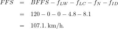
 | (6) |
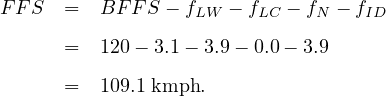
where, FFS = free flow speed (km/h), BFFS = base free flow speed (km/h), fLW = adjustment for lane width (km/h), fLC = adjustment for right shoulder clearance (km/h),fN = adjustment for no. of lanes (km/h), fID = adjustment for interchange density (km/h) Estimation of FFS for an existing or future freeway segment is accomplished adjusting a base free-flow speed downward to reflect the influence of four factors: lane width, lateral clearance, number of lanes, and interchange density. Thus, the analyst is required to select an appropriate BFFS as a starting point.
Adjustment for Lane Width The base condition for lane width is 3.6 m or greater. When the average lane width across all lanes is less than 3.6 m, the base free-flow speed (e.g., 120 km/h) is reduced. Adjustments to reflect the effect of narrower average lane width are given in Table 1.
| Lane Width (m) | fLW(km/h) |
| 3.6 | 0.0 |
| 3.5 | 1.0 |
| 3.4 | 2.1 |
| 3.3 | 3.1 |
| 3.2 | 5.6 |
| 3.1 | 8.1 |
| 3.0 | 10.6 |
Adjustment for Lateral Clearance Base lateral clearance is 1.8 m or greater on the right side and 0.6 m or greater on the median or left side, measured from the edge of the paved shoulder to the nearest edge of the travelled lane. When the right-shoulder lateral clearance is less than 1.8 m, the BFFS is reduced. Adjustments to reflect the effect of narrower right-shoulder lateral clearance are given in Table 2.
| Right Shoulder | ||||
| Lateral | ||||
| Clearance (m) | 2 | 3 | 4 | ≥5 |
| ≥1.8 | 0.0 | 0.0 | 0.0 | 0.0 |
| 1.5 | 1.0 | 0.7 | 0.3 | 0.2 |
| 1.2 | 1.9 | 1.3 | 0.7 | 0.4 |
| 0.9 | 2.9 | 1.9 | 1.0 | 0.6 |
| 0.6 | 3.9 | 2.6 | 1.3 | 0.8 |
| 0.3 | 4.8 | 3.2 | 1.6 | 1.1 |
| 0.0 | 5.8 | 3.9 | 1.9 | 1.3 |
Adjustment for Number of Lanes Freeway segments with five or more lanes (in one direction) are considered as having base conditions with respect to number of lanes. When fewer lanes are present, the BFFS is reduced. Table 3 provides adjustments to reflect the effect of number of lanes on BFFS. In determining number of lanes, only mainline lanes, both basic and auxiliary, should be considered.
| Number of Lanes | fN (km/h) |
| ≥ 5 | 0.0 |
| 4 | 2.4 |
| 3 | 4.8 |
| 2 | 7.3 |
Adjustment for Interchange Density The base interchange density is 0.3 interchanges per kilometer, or 3.3-km interchange spacing. Base free-flow speed is reduced when interchange density becomes greater. Adjustments to reflect the effect of interchange density are provided in Table 4. Interchange density is determined over a 10-km segment of freeway (5 km upstream and 5 km downstream) in which the freeway segment is located. An interchange is defined as having at least one on-ramp. Therefore, interchanges that have only off-ramps would not be considered in determining interchange density. Interchanges considered should include typical interchanges with arterial or highways and major freeway-to-freeway interchanges.
| Interchanges per km | fID (km/h) |
| ≤ 0.3 | 0.0 |
| 0.4 | 1.1 |
| 0.5 | 2.1 |
| 0.6 | 3.9 |
| 0.7 | 5.0 |
| 0.8 | 6.0 |
| 0.9 | 8.1 |
| 1.0 | 9.2 |
| 1.1 | 10.2 |
| 1.2 | 12.1 |
Level of service on the basis of density can be calculated using the equation 7
 | (7) |
Where, D = density (pc/km/ln), V p= flow rate (pc/h/ln), S = average passenger car speed (km/h). The density of the traffic stream can be used to determine the level of service of a freeway segment. Level-of-service thresholds based on density for a basic freeway segment are summarized in the Table 5 shown below.
| LOS | Density Range (pc/km/ln) |
| A | 0 - 7 |
| B | >7 - 11 |
| C | >11 - 16 |
| D | >16 - 22 |
| E | >22 - 28 |
| F | >28 |
Consider an existing four lane freeway in rural area, having very restricted geometry with rolling terrain. Peak hour volume is 2000 veh/h with 5% trucks. The traffic is commuter type with peak hour factor 0.92 and interchange density as 0.6 interchanges per kilometer. Freeway consists of two lanes in each direction of 3.3 m width with lateral clearance of 0.6 m. Find the LOS of freeway during peak hour.
Solution Assumptions: Assume 0 percent buses and RVs since none are indicated. Assume BFFS of 120 km/h for rural areas. Since the freeway is in a rural area assume that the number of lanes does not affect free-flow speed. Assume fp = 1.00 for commuter traffic. We can get the corresponding values of adjustment factors from the tables as - fLW=3.1, fLC=3.9, fID=3.9 and fN=0.
Step 1 Find fHV using equation 3 as given below -
Step 2 Convert volume (veh/h) to flow rate (pc/h/ln) using equation as given below

Step 3 Compute free-flow speed from equation 6 as given below and putting the respective values of adjustment factors we get FFS as
Step 4 Determine the density using the equation 7 as -

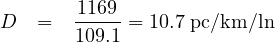
Step 5 Find Level of service, for the calculated value of density we can get the level of service from the LOS table. i.e for D = 10.7 pc/km/ln we get LOS = B
A new suburban freeway is designed in the level terrain. Peak hour volume is 4,000 veh/h and the flow consists of 15% trucks and 3% recreational vehicles (RV’s). The traffic is commuter type with peak hour factor 0.85 and interchange density as 0.9 interchanges per kilometer. Lane width is proposed to be 3.6 m with lateral clearance of 1.8 m. How many lanes are needed to provide LOS C during the peak hour?
Solution Assumptions: Assume BFFS of 120 km/h. Since the freeway is being designed in a suburban area assume that the number of lanes affects free-flow speed. For commuter traffic we can take fp = 1.00. We can get the corresponding values of adjustment factors from the tables as - fLW = 0,fLC = 0,fID = 8.1 and fN = 4.8.
Step 1 Find fHV using equation 3 as given below:
Step 2 Convert volume (veh/h) to flow rate (pc/h/ln) using equation 2. Consider a four lane option, for four lane N = 2, keeping value of fHV and N in equation 2 we get V p as:
Step 4 Consider a six lane option
Step 5 Compute FFS for a six-lane freeway from equation 6 and putting the respective values of adjustment factors we get FFS as:
Step 6 Determine density from equation 7

Step 7 Check the LOS, for the calculated value of density we can get the level of service from the LOS table; i.e for D = 15.8 pc/km/ln we get LOS = C. Hence number of lanes to be provided to satisfy LOS C during peak hour = 6.
Weaving is defined as the crossing of two or more traffic streams travelling in the same general direction along a significant length of highway without the aid of traffic control devices (with the exception of guide signs). Weaving segments are formed when a merge area is closely followed by a diverge area, or when an on-ramp is closely followed by an off-ramp and the two are joined by an auxiliary lane.
Weaving segments require intense lane-changing maneuvers as drivers must access lanes appropriate to their desired exit points. Thus, traffic in a weaving segment is subject to turbulence in excess of that normally present on basic freeway segments. The turbulence presents special operational problems and design requirements. Fig. 8 shows the simple weaving segment formed by a single merge point followed by a single diverge point. Multiple weaving segments may be formed where one merge is followed by two diverge points or where two merge points are followed by one diverge point.
The most critical aspect of operations within a weaving segment is lane changing. Weaving vehicles, which must cross a roadway to enter on the right and leave on the left, or vice versa, accomplish these maneuvers by making the appropriate lane changes. The configuration of the weaving segment (i.e., the relative placement of entry and exit lanes) has a major effect on the number of lane changes required of weaving vehicles to successfully complete their maneuver. There is also a distinction between lane changes that must be made to weave successfully and additional lane changes that are discretionary (i.e., are not necessary to complete the weaving maneuver). The former must take place within the confined length of the weaving segment, whereas the latter are not restricted to the weaving segment itself. There are three major categories of weaving configurations: Type A, Type B, and Type C.
The identifying characteristic of a Type A weaving segment is that all weaving vehicles must make one lane change to complete their maneuver successfully. All of these lane changes occur across a lane line that connects from the entrance gore area directly to the exit gore area. Such a line is referred to as a crown line. Type A weaving segments are the only such segments to have a crown line.
The most common form of Type A weaving segment is shown in Fig. 9. The segment is formed by a one-lane on-ramp followed by a one-lane off-ramp, with the two connected by a continuous auxiliary lane. The lane line between the auxiliary lane and the right-hand freeway lane is the crown line for the weaving segment. All on-ramp vehicles entering the freeway must make a lane change from the auxiliary lane to the shoulder lane of the freeway. All freeway vehicles exiting at the off-ramp must make a lane change from the shoulder lane of the freeway to the auxiliary lane. This type of configuration is also referred to as a ramp-weave.
Fig. 10 illustrates a major weaving segment that also has a crown line. A major weaving segment is formed when three or four of the entry and exit legs have multiple lanes. As in the case of a ramp-weave, all weaving vehicles, regardless of the direction of the weave, must execute one lane change across the crown line of the segment.
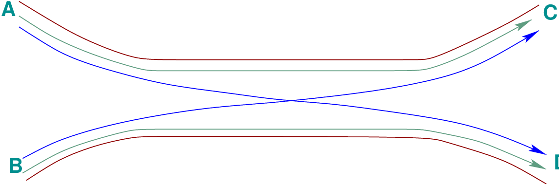
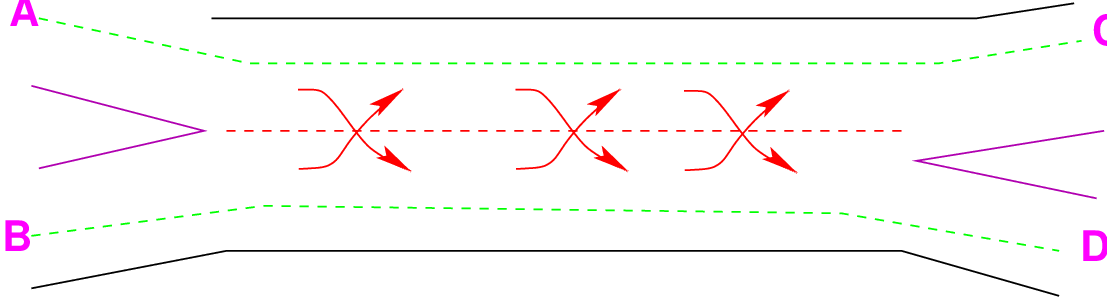
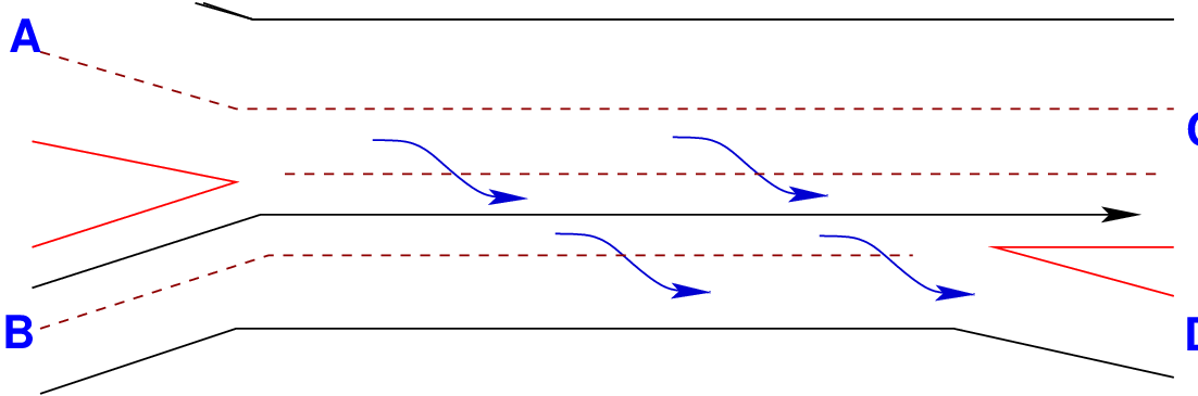
Type B weaving segments are shown in Figs. 11 to 13. All Type B weaving segments fall into the general category of major weaving segments in that such segments always have at least three entry and exit legs with multiple lanes (except for some collector distributor configurations). It is the lane changing required of weaving vehicles that characterizes for the Type B configuration:
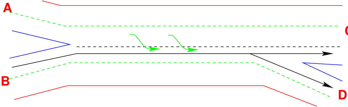
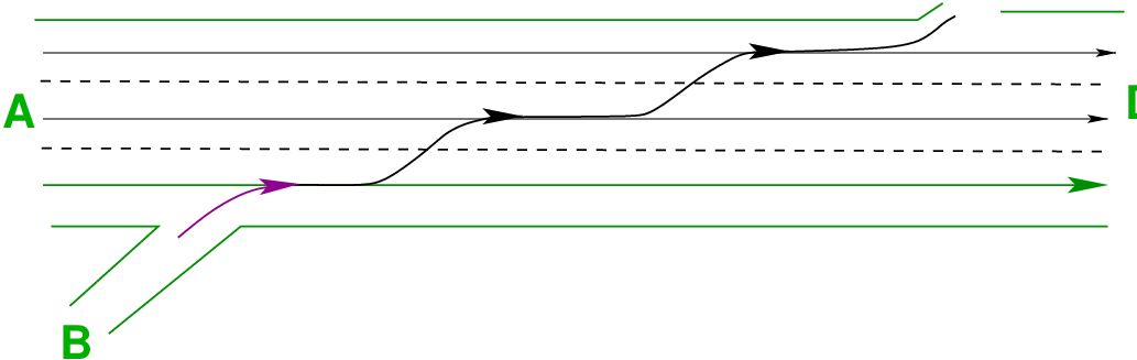
Figs. 11 to 13 show two Type B weaving segments. In both cases, Lane balance defined Movement B-C (entry on the right, departure on the left) may be made without executing any lane changes, whereas Movement A-D (entry on the left, departure on the right) requires only one lane change. Essentially, there is a continuous lane that allows for entry on the right and departure on the left.
In Fig. 11 this is accomplished by providing a diverging lane at the exit gore. From this lane, a vehicle may proceed down either exit leg without executing a lane change. This type of design is also referred to as lane balanced, that is, the number of lanes leaving the diverge is one more than the number of lanes approaching it.
In Fig. 12 the same lane-changing scenario is provided by having a lane from Leg A merge with a lane from Leg B at the entrance gore. This is slightly less efficient than providing lane balance at the exit gore but produces similar numbers of lane changes by weaving vehicles.
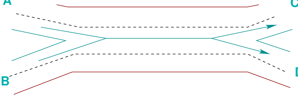
The configuration shown in Fig. 13 is unique, having both a merge of two lanes at the entrance gore and lane balance at the exit gore. In this case, both weaving movements can take place without making a lane change. Such configurations are most often found on collector-distributor roadways as part of an interchange.
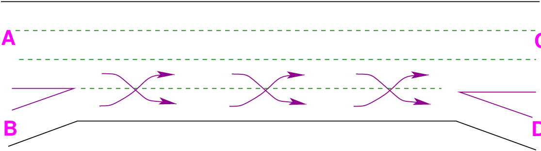
Type C weaving segments are similar to those of Type B in that one or more through lanes are provided for one of the weaving movements. The distinguishing characteristic of a Type C weaving segment is that the other weaving movement requires a minimum of two lane changes for successful completion of a weaving maneuver. Thus, a Type C weaving segment is characterized by the following:
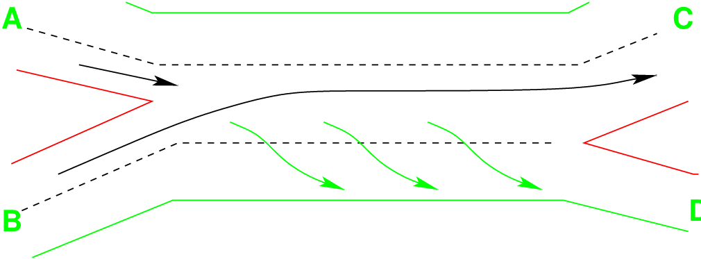
Figs. 14 to 15 shows two types of Type C weaving segments. In Fig. 14 Movement B-C
does not require a lane change, whereas Movement A-D requires two lane changes.
This type of segment is formed when there is neither merging of lanes at the entrance
gore nor lane balance at the exit gore, and no crown line exists. Although such a
segment is relatively efficient for weaving movements in the direction of the freeway
flow, it cannot efficiently handle large weaving flows in the other direction.
Fig. 15 shows a two-sided weaving segment. It is formed when a right-hand on-ramp is followed by a left-hand off-ramp, or vice versa. In such cases, the through freeway flow operates functionally as a weaving flow. Ramp-to-ramp vehicles must cross all lanes of the freeway to execute their desired maneuver. Freeway lanes are, in effect, through weaving lanes, and ramp-to-ramp vehicles must make multiple lane changes as they cross from one side of the freeway to the other.
The configuration of the weaving segment has a marked effect on operations because of its
influence on lane-changing behavior. A weaving segment with 1,000 veh/h weaving across
1,000 veh/h in the other direction requires at least 2,000 lane changes per hour in a Type A
segment, since each vehicle makes one lane change. In a Type B segment, only one
movement must change lanes, reducing the number of required lane changes per hour to
1,000. In a Type C segment, one weaving flow would not have to change lanes, while the
other would have to make at least two lane changes, for a total of 2,000 lane changes per
hour.
Configuration has a further effect on the proportional use of lanes by weaving and
lanes non weaving vehicles. Since weaving vehicles must occupy specific lanes to
efficiently complete their maneuvers, the configuration can limit the ability of weaving
vehicles to use outer lanes of the segment. This effect is most pronounced for Type A
segments, because weaving vehicles must primarily occupy the two lanes adjacent to the
crown line. It is least severe for Type B segments, since these segments require
the fewest lane changes for weaving vehicles, thus allowing more flexibility in lane
use.
Freeways are most efficient type of highway. Level of service (LOS) is a quality measure describing operational conditions within a traffic stream of freeways. Prevailing roadway, traffic and control conditions define capacity; these conditions should be reasonably uniform for any section of freeway analysed. Freeway management system works for smooth operations of freeway.
I wish to thank several of my students and staff of NPTEL for their contribution in this lecture. I wish to thank specially my student Mr. Amit Kumar for his assistance in developing the lecture note, and my staff Ms. Reeba in typesetting the materials. I also appreciate your constructive feedback which may be sent to tvm@civil.iitb.ac.in
Prof. Tom V. Mathew
Department of Civil Engineering
Indian Institute of Technology Bombay, India
_________________________________________________________________________
Wednesday 27 September 2023 10:44:33 PM IST