Ramp Metering

Lecture Notes in Transportation Systems Engineering

Prof. Tom V. Mathew

PDF for Online View or PDF for Print
(PDF for IITB students and is password protected)

1 Introduction
1.1 Objectives
1.2 Benefits
2 Metering strategies
2.1 Single-lane one car per green
2.2 Single-lane multiple cars per Green
2.3 Dual-lane metering
2.4 Quality of metering
3 Design of ramp metering
3.1 Minimum stopping distance to the back of queue
3.2 Storage distance
3.3 Distance from meter to merge
4 Ramp design methodology
5 Merging influence area
5.1 Predicting entering flow
5.2 Determining capacity
5.3 Determining LOS
  5.3.1 Numerical example
6 Diverge influence area
6.1 Predicting entering flow
6.2 Determining capacity
6.3 Determining LOS
  6.3.1 Numerical example
7 Fixed, reactive and predictive systems
7.1 Pre-timed (fixed) systems
7.2 Traffic responsive systems
  7.2.1 Local traffic responsive
  7.2.2 System-wide traffic responsive
8 Summary
Exercises
References
Acknowledgments

______________________________________________________________________

1 Introduction

Ramp metering can be defined as a method by which traffic seeking to gain access to a busy highway is controlled at the access point via traffic signals. This control aims at maximize the capacity of the highway and prevent traffic flow breakdown and the onset of congestion. Ramp metering is the use of traffic signals to control the flow of traffic entering a freeway facility. Ramp metering, when properly applied, is a valuable tool for efficient traffic management on freeways and freeway networks.

1.1 Objectives

The objectives of ramp metering includes:

Controlling the number of vehicles that are allowed to enter the freeway,
Reducing freeway demand, and
Breaking up of the platoon of vehicles released from an upstream traffic signal.

Figure 1 given below is a typical example of ramp metering. The signal placed at the ramp, controls the traffic flow which can enter the freeway through merge lane. Vehicle detectors are also shown at the downstream end of the freeway.

Figure 1: Schematic diagram of ramp metering

1.2 Benefits

Ramp metering has many positive benefits in freeway management with in measurable parameters such as reduced delay, reduced travel time, reduced accident risk and increased operating speed. The typical advantages are:

Improved System Operation: Ramp metering essentially aims to control the access to a freeway to reduce congestion, freeway delay and ultimately overall delay. Although several ramp metering strategies are available with individual pros and cons, overall, ramp metering helps to break up platoons of vehicles from entering a freeway and causing turbulence, reduces delay due to random access and defers if not eliminates the onset of congestion.
Improved Safety: Ramp areas are accident prone areas due to unmanaged merging and diverging. Ramp metering makes merging and diverging operation to a freeway smooth and controlled, reducing the risk of accidents arising out of sudden driver decisions. Random entry of platoons is also prevented which decreases the risk of accidents at merge or diverge areas.
Reduced vehicle operating expense and emission: Ramp metering essentially reduces the number of stops and delays for the freeway as well as the ramps. This in turn reduces the fuel consumption and emission for a vehicle.

2 Metering strategies

Metering strategies can be defined as the approach used to control the traffic the flow on the ramps. Three Ramp metering strategies are available to control the flow on the ramps which can enter the busy freeway. Capacity of an uncontrolled single-lane freeway entrance ramp is 1800 to 2200 vehicles per hour (VPH). Since Ramp metering is a traffic flow controlling approach it decreases the capacity of the ramps. Three ramp-metering strategies are as follows:

2.1 Single-lane one car per green

Single-lane one car per green ramp metering strategy allows only one car to enter the freeway during each signal cycle. The salient features of this strategy are:

The length of green plus yellow indications is set to ensure sufficient time for one vehicle to cross the stop line. The length of red interval should be sufficient to ensure that the following vehicle completely stops before proceeding.
A typical cycle length is taken as, the smallest possible cycle is 4 seconds with 1 second green, 1 second yellow, and 2 seconds red. This produces a meter capacity of 900 VPH.
A more reasonable cycle is around 4.5 seconds, obtained by increasing the red time to 2.5 seconds. This increase in red would result in a lower meter capacity of 800 VPH.

2.2 Single-lane multiple cars per Green

Single-Lane Multiple Cars per Green is also known as Platoon metering, or bulk metering. This approach allows two or more vehicles to enter the freeway during each green indication. The most common form of this strategy is to allow two cars per green. The salient features of this type of ramp metering are:

Three or more cars can be allowed; however, this will sacrifice the third objective(breaking up large platoons).
Furthermore, contrary to what one might think, bulk metering does not produce a drastic increase in capacity over a single-lane one car per green operation. This is because this strategy requires longer green and yellow times as ramp speed increases, resulting in a longer cycle length. Consequently, there are fewer cycles in one hour.
Two cars per green strategy requires cycle lengths between 6 and 6.5 seconds and results in metering capacity of 1100 to 1200 VPH. This analysis illustrates that bulk metering does not double capacity and this finding should be noted.

2.3 Dual-lane metering

In dual lane metering two lanes are required to be provided on the ramp in the vicinity of the meter which necks down to one lane at the merge. The salient features of this type of ramp metering are:

In this strategy, the controller displays the green-yellow-red cycle for each lane.
Synchronized cycles are used such that the green indications never occur simultaneously in both lanes.
The green indications are timed to allow a constant headway between vehicles from both lanes. Dual-lane metering can provide metering capacity of 1600 to 1700 VPH.
In addition, dual-lane ramps provide more storage space for queued vehicles.

2.4 Quality of metering

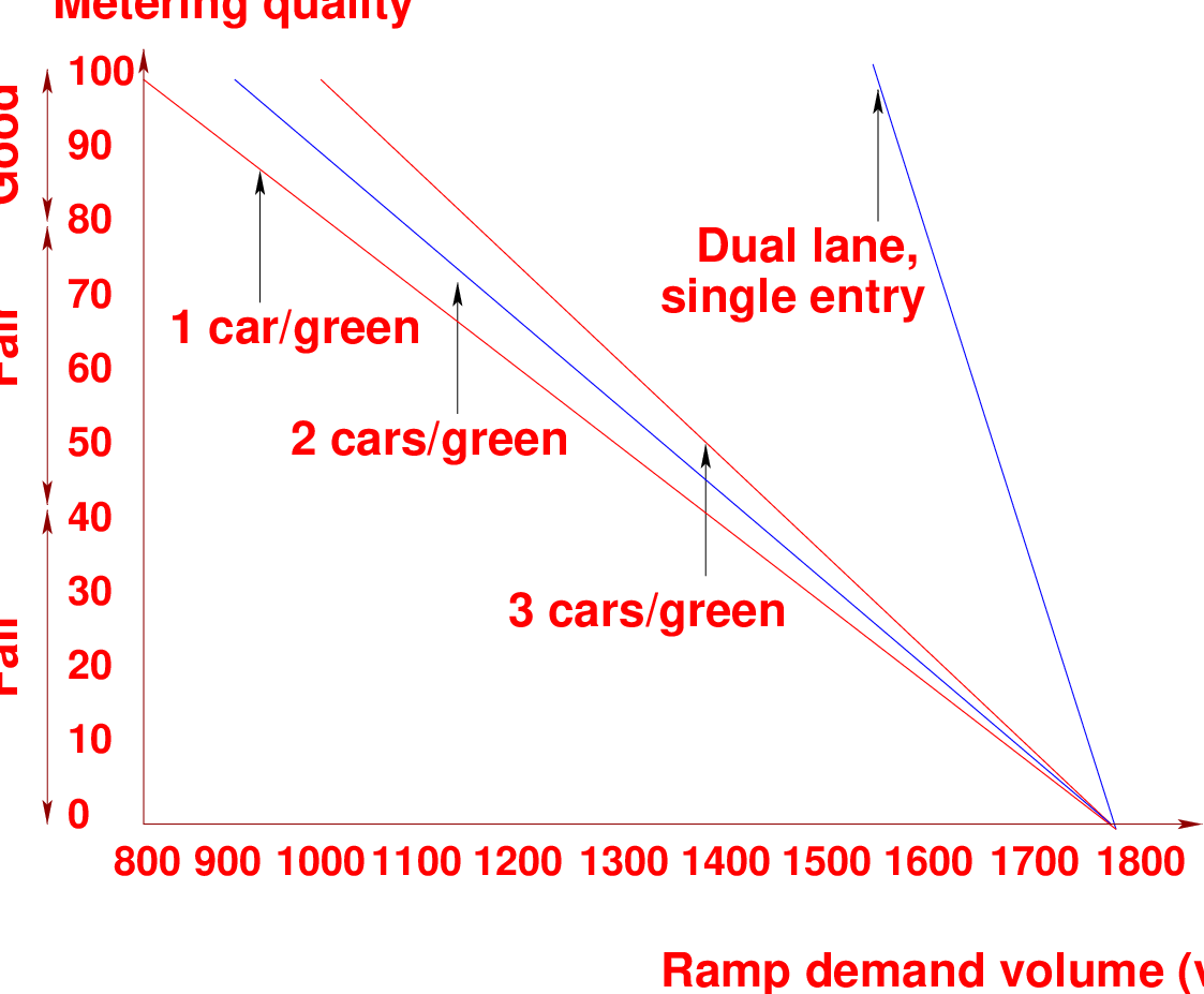
The quality of ramp metering essentially implies the efficiency of handling the flow and reducing unnecessary delays through metering strategies. For a ramp meter to produce the desired benefits, the engineer should select a metering strategy appropriate for the current or projected ramp demand. The ramp width will depend on this selection. The following fig. 2 shows the metering availability (percent of time the signal is metering) of the three metering strategies for a range of ramp demand volumes.

Figure 2: Comparison of metering quality of different approaches with Ramp demand volume

In Figure 2, if the flow on a single lane ramp which has Single-Lane One Car per Green approach is 1000 vph, then the metering availability is only 80 percent since the metering approach installed has the capacity of 800 vph. Therefore metering availability decreases as the traffic flow increases. If the flow is around 1600 vph then Dual-Lane Metering gives 100 percent metering availability. Thus it is imperative to select the metering strategy based on the flow and accordingly select the required ramp width.

3 Design of ramp metering

There are some considerations to be taken into account before designing and installing a ramp meter. Installation of a ramp meter to achieve the desired objectives requires sufficient room at the entrance ramp. The determination of minimum ramp length to provide safe, efficient, and desirable operation requires careful consideration of several elements described below:

Sufficient room must be provided for a stopped vehicle at the meter to accelerate and attain safe merge speeds.
Sufficient space must be provided to store the resulting cyclic queue of vehicles without blocking an upstream signalized intersection.
Sufficient room must be provided for vehicles discharged from the upstream signal to safely stop behind the queue of vehicles being metered.

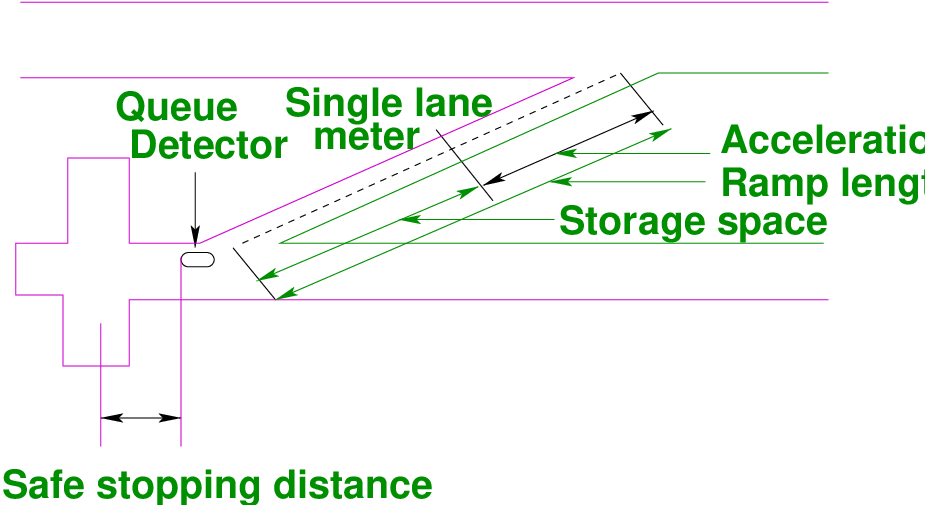
Provision for the distances mentioned is an integral part of ramp design. Figure 3 illustrates the requirements for the different types of distances explained above.

3.1 Minimum stopping distance to the back of queue

Sufficient stopping distance is required to be provided prior to entry to the ramp. Motorists leaving an upstream signalized interchange will likely encounter the rear end of a queue as they proceed toward the meter. Adequate maneuvering and stopping distances should be provided for both turning and frontage road traffic. This stopping distance calculated similar to the stopping sight distance which is a combination of the brake distance and lag distance travelled by a vehicle before stopping. The equation to calculate the minimum stopping distance is given below:

v2 X = vt + 2gf-

(1)

where, X is the stopping distance in meters, v is the velocity of the vehicle in m/sec, t is the time in seconds, g is the gravity coefficient in m∕sec², f is the friction coefficient. This is the minimum distance to be provided from the back of the queue for safe stopping of vehicles approaching the ramp.

Figure 3: Components of Ramp design criteria

Figure 3 shows Safe stopping distance, storage distance and acceleration distance which are respective three criteria for ramp design.

3.2 Storage distance

The storage distance is required to store the vehicles in queue to a ramp meter. The queue detector controls the maximum queue length in real-time. Thus, the distance between the meter and the queue detector defines the storage space. The following generalized spacing model can be used to determine the single-lane storage distance:

2 L = aV - bV ∀ V ≤ 1600 vph

(2)

In this equation, L (in meters) is the required single-lane storage distance on the ramp when the expected peak-hour ramp demand volume is V vph and a, b are constants. This figure shows the requirements for three metering strategies:

Single-lane with single vehicle release per cycle.
Single-lane with bulk metering (three vehicles per green).
Dual-lane metering assuming single-line storage.

Figure 4: Variation of distance to meter with Ramp demand volume for different strategies of Ramp metering

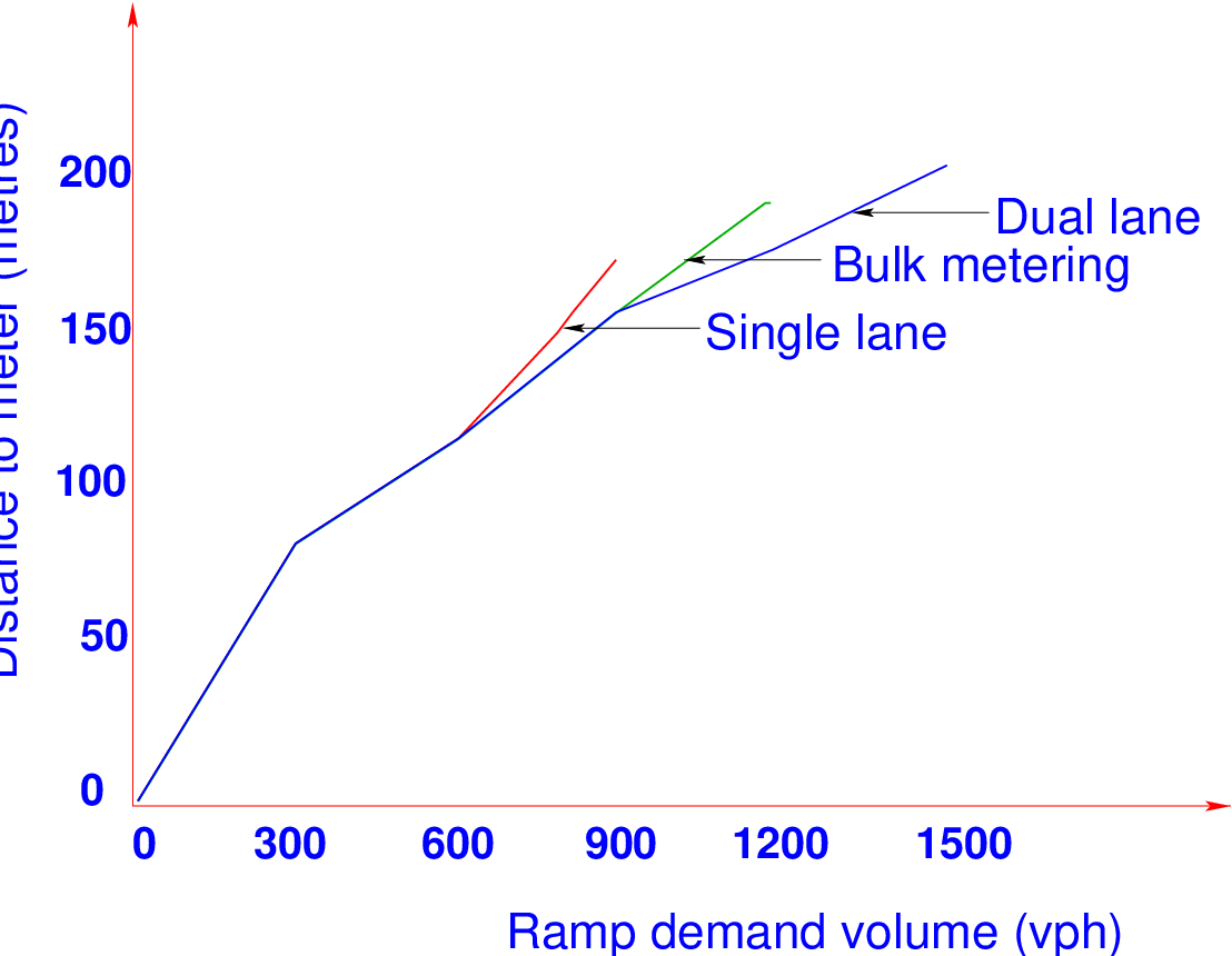
In the Figure 4 the curve is shown for the variation of storage distance i.e. distance to meter with ramp demand volume for different strategy used for Ramp metering.

3.3 Distance from meter to merge

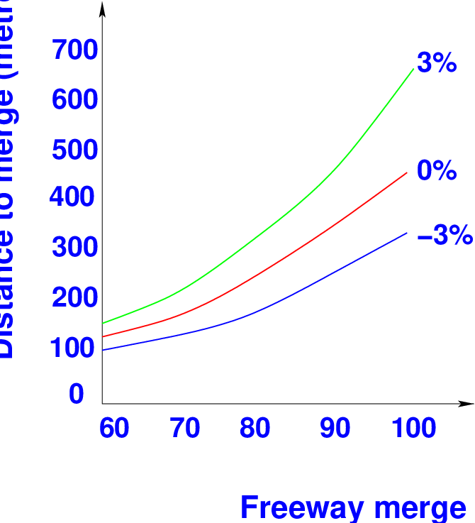
The distance from meter to merge is provided so that vehicles can attain a suitable merging speed after being discharged from the ramp meter. AASHTO provides speed-distance profiles for various classes of vehicles as they accelerate from a stop to speed for various ramp grades. Figure 5, given below provides similar acceleration distances needed to attain various freeway merging speeds based on AASHTO design criteria.

Figure 5: Acceleration length v/s merge speed for different strategies of Ramp metering

Table 1 provides the acceleration length for different merge speed and with ramps of different grade. The desired distances to merge increases with increasing freeway merge speed and the same ramp grade.

Table 1: Acceleration length of ramps


Merge speed	Ramp Grade (%)

(kmph)	-3	0	+3

60	90	112	150

70	127	158	208

80	180	228	313

90	248	323	466

100	331	442	665

4 Ramp design methodology

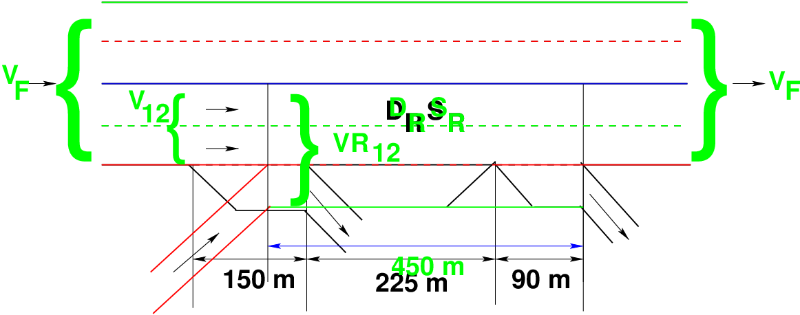
To model the ramp influence area, a length of 450 m just upstream (for off ramp) and downstream (for on ramp) is considered to be affected. The input data required is the geometric data of the freeway and the ramp and the demand flow. The three steps of design are:

The flow entering lanes 1 and 2 of the freeway upstream of merge area or diverge area is first determined.
The capacity of the freeway, ramp and merge and diverge areas are determined and checked with limiting values to determine the chance of occurrence of congestion.
The density in the ramp influence area is then found out and depending on the value f this variable, the level of service is determined.

From design point of view analysis of merge area and diverge area are treated separately but follows the same basic principle already explained.

5 Merging influence area

The Merging influence area is the area where increase in local density, congestion, and reduced speeds is generally observed due to merging traffic from ramps. The ramp contributing traffic to the freeway is called an ON ramp. The analysis of the merging influence area is done to find out the level of service of the ON ramp (Figure 6). The analysis of merge area is done in following three primary steps:

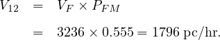
Figure 6: Schematic view of a typical merging area

5.1 Predicting entering flow

The first step of the merge area analysis is to predict the flow entering lanes 1and 2 of the freeway (V ₁₂). The terms used in above figure are explained below. V ₁₂ is influenced by the following factors:

Total freeway flow approaching merge area (V _F) (pc/h): The total approach flow is the most important influencing factor for the flow remaining in lanes 1 and 2 of the freeway.
Total Ramp Flow (V _R): This is the total flow on the ramp which ultimately enters the freeway to merge with existing flow.
Total length of acceleration lane: A longer acceleration lane reduces the turbulence and hence the density in the influence area of the ramp. The flow in the lanes 1 and 2 thus are higher.
Free- flow speed of ramp at point of merge area: Higher the free flow speed of ramp vehicles, vehicles on freeway tend to move away from merging flow to avoid high speed turbulence.

HCM 2000 provides model for predicting V ₁₂ at on-ramps as given below:

V12 = VF × PF M

(3)

where V ₁₂ is the flow rate in lane 1 and 2 of freeway entering ramp influence area (pc/h), V _F is the total freeway flow approaching merge area, and P_FM is the Proportion of approaching freeway flow remaining in lanes 1 and 2 immediately upstream of merge. For four lanes freeway (2 lanes in each direction) P_FM = 1.00

5.2 Determining capacity

Determining the capacity of the merge area is the second step of the analysis. The capacity of a merge area is determined by the capacity of the downstream freeway segment. Thus, the total flow arriving on the upstream freeway and the on-ramp cannot exceed the basic freeway capacity of the departing downstream freeway segment.

vR12 = v12 + vR

(4)

Two conditions may occur in a given analysis:

The total departing freeway flow, given as V = v_F + v_R, is greater than the capacity of the down steam freeway segment, and hence the LOS is F and queuing is expected on the freeway.
Flow entering the ramp influence area exceeds its capacity but total departing freeway flow is within capacity. This may result in in local high densities and queuing is not expected on the freeway.

5.3 Determining LOS

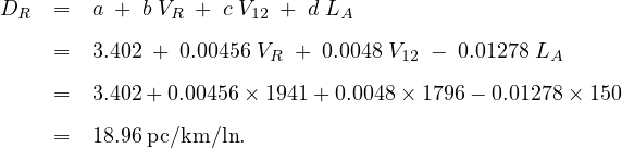
Determining the level of service (LOS) of the merge area is the third step in merge area analysis. LOS depends on the density in the influencing area. HCM 2000 provides the equation to estimate the density in the merge influence area.

DR = a+ b VR + c V12 + d LA

(5)

where, D_R is the density of merge influence area (pc/km/ln), V _R is the on-ramp peak 15-min flow rate (pc/h), L_A is the length of acceleration lane (m), V ₁₂ is the flow rate entering ramp influence area (pc/h), and a, b, c, and d are constants.

Table 2: LOS criteria for merge and diverge areas


LOS	Density (pc/km/lane)

A	≥ 6

B	6 - 12

C	12 - 17

D	17 - 22

E	> 22

F	Demands exceeds capacity

5.3.1 Numerical example

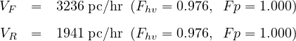
Consider a single lane on-ramp to a six-lane freeway. The length of the acceleration lane is 150 m. What is the LOS during the peak hour for the first on-ramp? Given that the peak hour factor is 0.95, the heavy vehicle adjustment factor is 0.976, the driver adjustment factor is 1.0 and proportion of approaching freeway flow remaining is 55.5%? The freeway volume is 3000 veh/hr and the on-ramp volume is 1800 veh/hr.

Solution

Convert volume to flow rate: Convert volume in (veh/hr) to flow rate (pc/hr) using
$V vi = -------i------- PHF × Fhv × Fp$

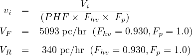
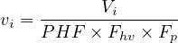where, vi is the flow rate in pc/hr for direction i, Vi is the hourly volume in veh/hr for direction i, PHF is the peak hour factor, and Fhv is the adjustment factor for heavy vehicles, and Fp is the adjustment factor for driver population.
$VF = 3236 pc∕hr (Fhv = 0.976, Fp = 1.000) VR = 1941 pc∕hr (Fhv = 0.976, Fp = 1.000)$
Compute V ₁₂ as:
$V12 = VF × PF M = 3236 × 0.555 = 1796 pc∕hr.$
Compute density at ramp influence area using equation:
$DR = a + b VR + c V12 + d LA = 3.402 + 0.00456 VR + 0.0048 V12 - 0.01278 LA = 3.402+ 0.00456× 1941+ 0.0048 × 1796 - 0.01278× 150 = 18.96 pc∕km ∕ln.$
Compute LOS For D_R=18.96 pc/km/ln, the LOS = D from the LOS table above.

6 Diverge influence area

The Diverging influence area is the area where increase in local density, congestion, and reduced speeds is generally observed due to diverging traffic to ramps. The ramp which diverge traffic to the ramp is called an OFF ramp. The analysis of the diverging influence area is done to find out the level of service of the OFF ramp. The analysis of diverge area is done in following three primary steps:

6.1 Predicting entering flow

The first step is same as that of merge area analysis. The flow in lanes 1 and 2 of the freeway is first predicted. However, there are two major differences in the analysis of diverge area.

First, approaching flow V ₁₂ is measured for a point immediately upstream of the deceleration lane.
Second, V ₁₂ includes V _R at the diverge area. V12 is the flow rate entering ramp influence area (pc/h), and vR is the Off-ramp demand flow rate (pc/h).

Figure 7: Typical diverging area diagram

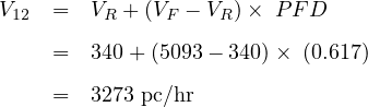
The general model given by HCM 2000 treats V ₁₂ as the sum of the off-ramp flow plus a proportion of the through freeway flow.

V12 = VR +(VF - VR)× PFD

(6)

where, V ₁₂ is the flow rate in lanes 1 and 2 of freeway upstream of diverge area in (pc/hr), V _F is the freeway demand flow rate immediately upstream of diverge in (pc/h), and P_FD is the proportion of through freeway flow remaining in lanes 1 and 2 immediately upstream of diverge. For four lanes freeway (2 lanes in each direction) P_FD is 1.00.

6.2 Determining capacity

As in the merge area analysis, determining the capacity is the second step of the diverge area analysis. Three limiting values should be checked:

Total flow that can depart from the diverge: this is limited by the capacity of the lanes in the freeway prior to approach of the diverge.
The capacities of the departing freeway leg or legs or ramp or both. This is the most important of the three as generally diverge areas fail due to failure of one or more exit legs..
V ₁₂ (approaching flow) prior to deceleration lane: this flow also includes the off-ramp flow and must be checked against capacity.

6.3 Determining LOS

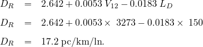
Determine the level of service (LOS) of the diverge area is the third step of the diverge area analysis. LOS criteria for diverge area are based on density in the diverge influence area. HCM 2000 provides the equation to estimate the density in the merge influence area.

DR = a + b V12 + cLD

(7)

where, D_R is the density of diverge influence area (pc/km/ln), V ₁₂ is the flow rate entering ramp influence area (pc/h), L_D is the length of deceleration lane(m), and a, b & c are constants. This equation is applicable only for under saturated conditions of flow. The density calculation is not done when either of the three capacities mentioned earlier are exceeded. In such cases, the LOS is assigned as F.

6.3.1 Numerical example

Consider an off-ramp (Single-lane) pair, 225 meters apart, from a six lane freeway. The length of the first deceleration lane is 150m and that of the second deceleration lane is 90 m. What is the LOS during the peak hour for the first off-ramp given that the peak hour factor is 0.95, the heavy vehicle adjustment factor is 0.93, the driver adjustment factor is 1.0 and the proportion of through freeway flow remaining is 61.7%? The freeway volume is 4500 veh/hr and the first off-ramp volume is 300 veh/hr.

Figure 8: Numerical example

Solution

Convert volume to flow rate: Convert volume in veh/hr to flow rate in pc/hr as follows:
$v = --------Vi-------- i (PHF × Fhv × Fp ) VF = 5093 pc∕hr (Fhv = 0.930,Fp = 1.0) VR = 340 pc∕hr (Fhv = 0.930,Fp = 1.0)$
Compute V ₁₂ as below:
$V12 == V3R4 +0+(V(F50-93 V-R)3×40)P×F(D0.617) = 3273 pc∕hr$
Compute density at ramp influence area as below:
$DR = 2.642 + 0.0053 V12 - 0.0183 LD D = 2.642 + 0.0053× 3273- 0.0183 × 150 R DR = 17.2 pc∕km∕ln.$
Determine LOS: For D_R=17.2 pc/km/ln the LOS is D.

7 Fixed, reactive and predictive systems

There are two different metering approaches available. First is Pre-timed metering, which use fixed signal cycles. Second is Traffic responsive, which uses real time traffic data to calculate signal cycle lengths. Traffic responsive systems can be local or system-wide.

7.1 Pre-timed (fixed) systems

In the pre-timed ramp metering systems, the ramp signal operates with a constant cycle in accordance with a metering rate prescribed for the particular control period.. the salient features of this type of ramp metering are:

It is the simplest and least expensive form of ramp metering for construction and installation.
It is also the most rigid approach because it cannot make adjustments for real-time conditions including non-recurring congestion (i.e., congestion that occurs as a result of weather, collisions, etc.).
Th system being pre-timed, it is best used to address conditions that are predictable from day-today.
If there is no mainline or ramp detection, agencies must regularly collect data by alternative means in order to analyze traffic conditions on the freeway and determine the appropriate metering rates.
The metering operation will require frequent observation so that rates can be adjusted to meet traffic conditions which is a drawback.

7.2 Traffic responsive systems

In contrast to the pre-timed metering control, traffic-responsive metering is directly influenced by the mainline and ramp traffic conditions during the metering period. Metering rates are selected on the basis of real-time measurements of traffic variables indicating the current relation between upstream and downstream capacity. The salient features of this type of ramp metering system are:

This system uses freeway loop detectors or other surveillance systems to calculate or select ramp metering rates based on current freeway conditions.
It is generally considered to be five to ten percent better than those of pre-timed metering.
A traffic responsive approach can be used either locally or system-wide.

7.2.1 Local traffic responsive

Local ramp metering is employed when only the conditions local to the ramp (as compared with other ramps) are used to provide the metering rates. The salient features are:

Local traffic responsive metering approaches base metering rates on freeway conditions near the metered ramp.
This is used where the traffic congestion at a location can be reduced by the metering of a single ramp.
They are used as backups when system-wide algorithms fail.
Unlike pre-timed systems, local systems require surveillance of the freeway using traffic detectors.
Although, more capital costs are required to implement traffic responsive systems, they more easily adapt to changing conditions and can provide better results than their pre-timed counterparts.

7.2.2 System-wide traffic responsive

In most cases, it is preferable to meter a series of ramps in a freeway section in a coordinated fashion based on criteria that consider the entire freeway section. The strategy may also consider the freeway corridor consisting of the freeway section as well as the surface streets that will be affected by metered traffic. The salient features are:

This is used when there are multiple bottlenecks or locations of recurring congestion along a freeway.
This type of ramp metering is used to optimize traffic flow along a metered stretch of roadway, rather than at a specific point on the freeway (as is the case of local traffic responsive systems).
Like local traffic responsive systems, system-wide traffic responsive systems require data from ramp detectors and local freeway detectors.
In addition to these components, system-wide traffic responsive systems are unique in the fact that data is also needed from downstream detectors and/or upstream detectors at multiple locations, potentially from cross-street signal controllers, and from the central computer.
System-wide traffic responsive systems have the most complex hardware configuration compared to the other metering approaches discussed so far (i.e., pre-timed and local traffic responsive).

8 Summary

In this chapter we discussed ramp metering, different strategies of ramp metering, procedure to find out the level of service of on and off ramps, different kind of metering systems. From the analysis that we have done in this chapter we can say that the Ramp metering can result into increased freeway speed, decreased travel time, increase in freeway capacity, reduction in accidents and congestion, improved fuel economy and efficient use of capacity.

Exercises

Not Available

References

Ismail Chabini and Amedeo R Odoni. Transportation Flow Systems. MIT, 2019.
A Chaudhary and J Messer. Report on design criteria for ramp metering. Texas Transportation Institute, Texas, 2000.
Highway Capacity Manual. Transportation Research Board. National Research Council, Washington, D.C., 2000.
P Stewart. Ramp metering study. SIAS Limited, Dundee, UK, 2003.

Acknowledgments

I wish to thank several of my students and staff of NPTEL for their contribution in this lecture. I wish to thank specially my student Mr. Abhimanyu Jain for his assistance in developing the lecture note, and my staff Mr. Rayan in typesetting the materials. I also appreciate your constructive feedback which may be sent to tvm@civil.iitb.ac.in

Prof. Tom V. Mathew
Department of Civil Engineering
Indian Institute of Technology Bombay, India

_________________________________________________________________________

Wednesday 27 September 2023 10:44:47 PM IST