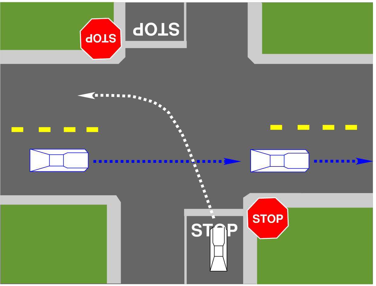
Figure 1: Example showing uncontrolled intersection
Uncontrolled intersections are the traffic junctions where there is no explicit traffic control measures are adopted. The important aspects that will be covered in this chapter are: the concept of two-way stop controlled intersection, all-way stop controlled intersection, gap acceptance, critical gap, follow-up time, potential capacity, and delay determination. These concepts are primarily adopted from Highway Capacity Manual.
An intersection is a road junction where two or more roads either meet or cross at grade. This intersection includes the areas needed for all modes of travel: pedestrian, bicycle, motor vehicle, and transit. Thus, the intersection includes not only the pavement area, but typically the adjacent sidewalks and pedestrian curb cut ramps.
All the road junctions designated for the vehicles to turn to different directions to reach their desired destinations. Traffic intersections are complex locations on any highway. This is because vehicles moving in different direction want to occupy same space at the same time. In addition, the pedestrians also seek same space for crossing. Drivers have to make split second decision at an intersection by considering his route, intersection geometry, speed and direction of other vehicles etc. A small error in judgment can cause severe accidents. It causes delay and it depends on type, geometry, and type of control. Overall traffic flow depends on the performance of the intersections. It also affects the capacity of the road. Therefore, both from the accident perspective and the capacity perspective, the study of intersections are very important by the traffic engineers. Intersection design can vary widely in terms of size, shape, number of travel lanes, and number of turn lanes. Basically, there are four types of intersections, determined by the number of road segments and priority usage.
At uncontrolled intersection the arrival rate and individuals drivers generally determine the manner of operation, while the resulting performance characteristics are derived from joint consideration of flow conditions and driver judgment and behavior patterns. In simplest terms, an intersection, one flow of traffic seeks gaps in the opposing flow of traffic.
At priority intersections, since one flow is given priority over the right of way it is clear that the secondary or minor flow is usually the one seeking gaps. By contrast at uncontrolled intersection, each flow must seek gaps in the other opposing flow. When flows are very light, which is the case on most urban and rural roads large gaps exist in the flows and thus few situation arise when vehicles arrive at uncontrolled intersection less than 10 second apart or at interval close enough to cause conflicts. However when vehicles arrive at uncontrolled intersection only a few second apart potential conflicts exist and driver must judge their relative time relationships and adjusts accordingly.
Generally one or both vehicles most adjust their speeds i.e. delayed somewhat with the closer vehicle most often taking the right of way; in a sense, of course, the earlier arriving vehicle has priority and in this instance when two vehicles arrive simultaneous, the rule of the road usually indicate priority for the driver on the right. The possibility of judgmental in these, informal priority situation for uncontrolled intersection is obvious. At an Uncontrolled intersection: Service discipline is typically controlled by signs (stop or yield signs) using two rules two way stop controlled intersection (TWSC) and all way stop controlled intersection (AWSC).
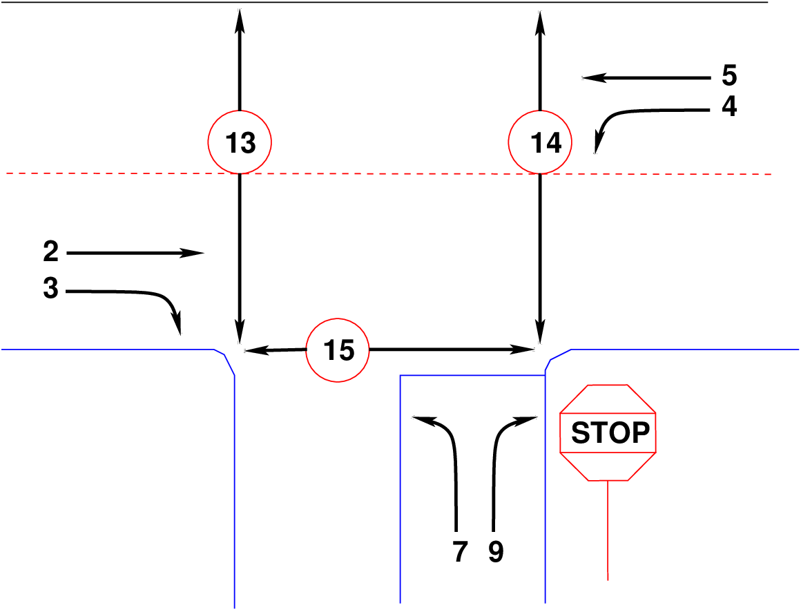
Researchers rely on many specific definitions to describe the performance of traffic operation systems. The clear understanding of such terminology is an important element is studying two-way stop-controlled (TWSC) traffic operation system characteristics; defined as: One of the uncontrolled intersections with stop control on the minor street shown in Fig. 2.
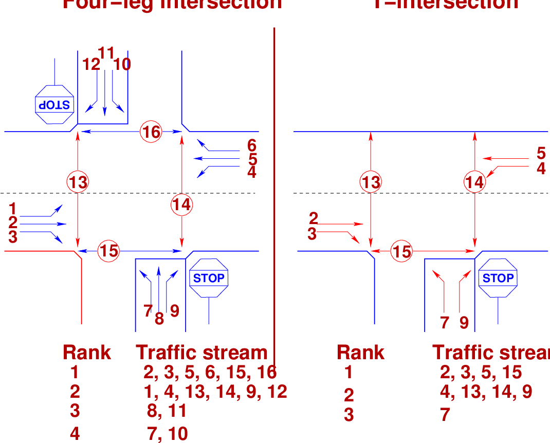
At TWSC intersections, the stop-controlled approaches are referred to as the minor street approaches; the intersection approaches that are not controlled by stop signs are referred to as the major street approaches. A three-leg intersection is considered to be a standard type of TWSC intersection if the single minor street approach is controlled by a stop sign. Three-leg intersections where two of the three approaches are controlled by stop signs are a special form of uncontrolled intersection control.
TWSC intersections assign the right-of-way among conflicting traffic streams according to the following hierarchy:
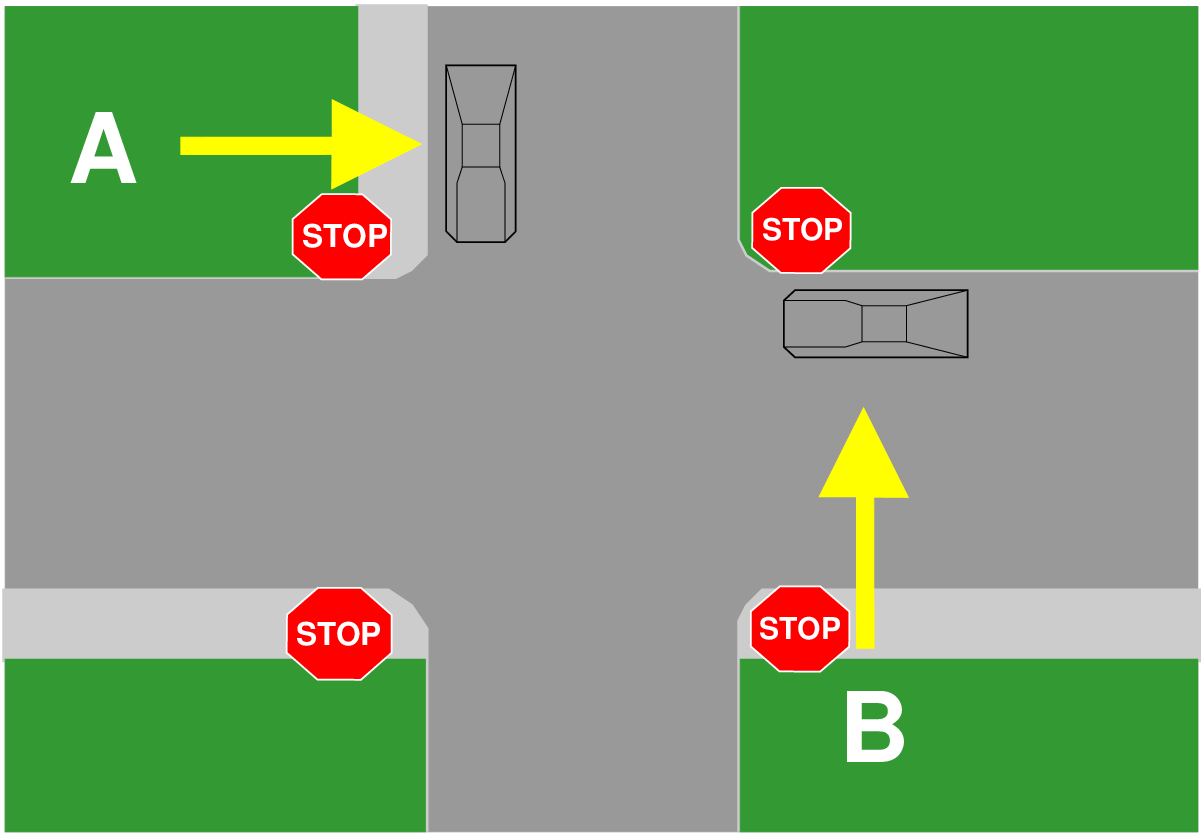
All-way-stop-controlled intersection (AWSC) are mostly used approaching from all directions and is required to stop before proceeding through the intersection as shown in Fig. 4. An all-way stop may have multiple approaches and may be marked with a supplemental plate stating the number of approaches.
The analysis of AWSC intersection is easier because all users must stop. In this type of intersection the critical entity of the capacity is the average intersection departure head way. Secondary parameters are the number of cross lanes, turning percentages, and the distribution volume on each approach. The first step for the analysis of capacity is select approach called subject approach the approach opposite to subject approach is opposing approach, and the approach on the side of the subject approach is are called conflicting approach.
AWSC intersections require every vehicle to stop at the intersection before proceeding. Since each driver must stop, the judgment as to whether to proceed into the intersection is a function of traffic conditions on the other approaches. If no traffic is present on the other approaches, a driver can proceed immediately after the stop is made. If there is traffic on one or more of the other approaches, a driver proceeds only after determining that there are no vehicles currently in the intersection and that it is the driver’s turn to proceed.
Gap acceptance is one of the most important components in microscopic traffic characteristic. The gap acceptance theory commonly used in the analysis of uncontrolled intersections based on the concept of defining the extent drivers will be able to utilize a gap of particular size or duration. A driver entering into or going across a traffic stream must evaluate the space between a potentially conflicting vehicle and decide whether to cross or enter or not. One of the most important aspects of traffic operation is the interaction of vehicles with in a single stream of traffic or the interaction of two separate traffic streams. This interaction takes place when a driver changes lanes merging in to a traffic stream or crosses a traffic stream. Inherent in the traffic interaction associated with these basic maneuvers is concept of gap acceptance.
The critical gap tcx for movement x is defined as the minimum average acceptable gap that allows intersection entry for one minor street or major street. The term average acceptable means that the average driver would accept or choose to utilize a gap of this size. The gap is measured as the clear time in the traffic stream defined by all conflicting movements. Thus, the model assumes that all gaps shorter than tcx are rejected or unused, while all gaps equal to or larger than tcx would be accepted or used. The adjusted critical gap tcx computed as follows.
 | (1) |
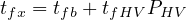
where, tcx is the critical gap for movement “x”, tcb is the base critical gap from Table. 1 tcHV is the adjustment factor for heavy vehicles PHV is the proportion of heavy vehicles tcG is the adjustment factor for grade G is the percent grade divided by 100, tcT is the adjustment factor for each part of a two-stage gap acceptance process, and t3LT is the critical gap adjustment factor for intersection geometry.
The follow up time tfx for movement “x” is the minimum average acceptable time for a second queued minor street vehicle to use a gap large enough admit two or more vehicles. Follow-up times were measured directly by observing traffic flow. Resulting follow-up times were analyzed to determine their dependence on different parameters such as intersection layout. This measurement is similar to the saturation flow rate at signalized intersection. Table. 1 and 2 shows base or unadjusted values of the critical gap and follow up time for various movements. Base critical gaps and follow up times can be adjusted to account for a number of conditions, including heavy - vehicle presence grade, and the existence of two stage gap acceptance. Adjusted Follow up Time computed as:
 | (2) |
where, tfx is the follow-up time for minor movement x tfb is the base follow-up time from table 1 tfHV is the adjustment factor for heavy vehicles, and PHV is the proportion of heavy vehicles for minor movement.
Base Critical Gap,tc,base (s) | Base Follow-up | ||
| Vehicle Movement | Two-Lane | Four-Lane | Time |
| Major Street | Major Street | tf,base (s) | |
| Left turn from major | 4.1 | 4.1 | 2.2 |
| Right turn from minor | 6.2 | 6.9 | 3.3 |
| Through traffic on minor | 6.5 | 6.5 | 4.0 |
| Left turn from minor | 7.1 | 7.5 | 3.5 |
| Adjustment | Values(s)
| |
| Factor | ||
| tcHV | 1.0 | Two-lane major streets |
| 2.0 | Four-lane major streets | |
| tcG | 0.1 | Movements 9 and 12 |
| 0.2 | Movements 7,8,10 and 11 | |
| 1.0 | Otherwise | |
| tcT | 1.0 | First or second stage of two-stage process |
| 0.0 | For one-stage process | |
| T3LT | 0.7 | Minor-street LT at T-intersection |
| 0.0 | Otherwise | |
| tfHV | 0.9 | Two-lane major streets |
| 1.0 | Four-lane major streets | |
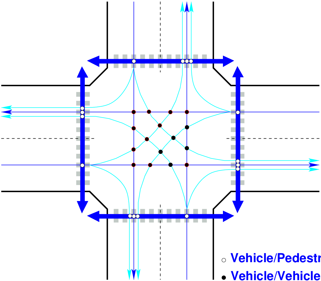
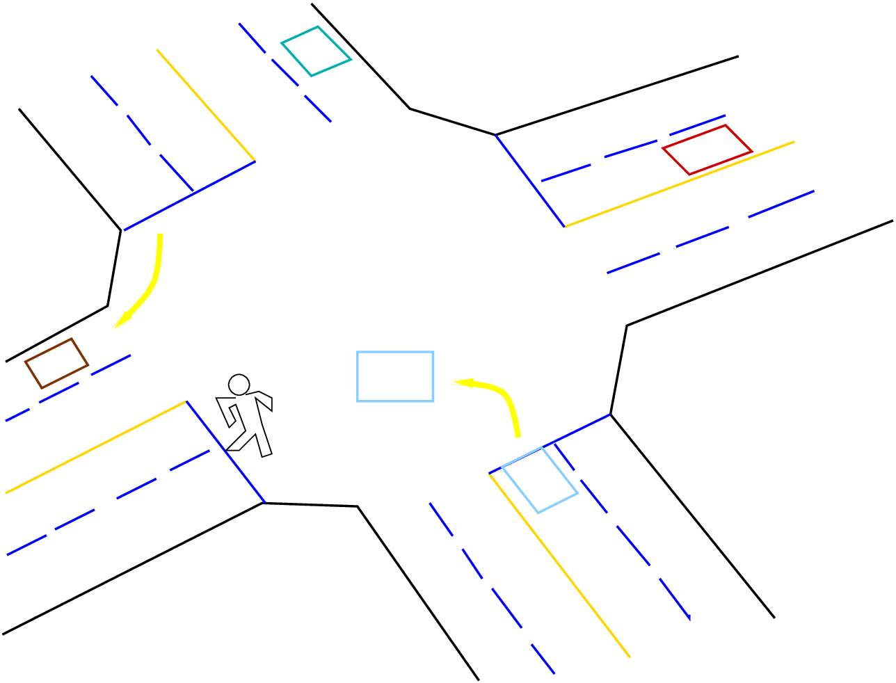
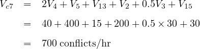
The traffic flow process at un-controlled intersection is complicated since there are many distinct vehicular movements to be accounted for. Most of this movements conflict with opposing vehicular volumes. These conflicts result in decreasing capacity, increasing delay, and increasing potentials for traffic accidents. Consider a typical four-legged intersection as shown in Fig. 5 The numbers of conflicts for competing through movements are 4, while competing right turn and through movements are 8. The conflicts between right turn traffics are 4, and between left turn and merging traffic are 4. The conflicts created by pedestrians will be 8 taking into account all the four approaches. Diverging traffic also produces about 4 conflicts. Therefore, a typical four legged intersection has about 32 different types of conflicts.
Conflicts at an intersection are different for different types of intersection. The essence of the intersection control is to resolve these conflicts at the intersection for the safe and efficient movement of both vehicular traffic and pedestrians. The movements for determining conflict in four legged intersection are:
Through this movements the conflict volume (V cx) for the given movement x is can be computed. As an example the formula of conflict volume for movement 7 for three legged intersection shown in Fig. 6 computed as:
 | (3) |
Capacity is defined as the maximum number of vehicles, passengers, or the like, per unit time, which can be accommodated under given conditions with a reasonable expectation of occurrence. Potential capacity describes the capacity of a minor stream under ideal conditions assuming that it is unimpeded by other movements and has exclusive use of a separate lane.
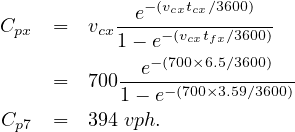
Once of the conflicting volume, critical gap and follow up time are known for a given movement its potential capacity can be estimated using gap acceptance models. The concept of potential capacity assumes that all available gaps are used by the subject movement i.e.; there are no higher priority vehicular or pedestrian movements and waiting to use some of the gaps it also assumes that each movement operates out of an exclusive lane. The potential capacity of can be computed using the formula:
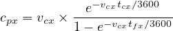 | (4) |
where, cpx is the potential capacity of minor movement x (veh/h), vcx is the conflicting flow rate for movement x (veh/h), tcx is the critical gap for minor movement x, and tfx is the follow-up time movement x.
Vehicles use gaps at a TWSC intersection in a prioritized manner. When traffic becomes congested in a high-priority movement, it can impede lower-priority movements that are streams of Ranks 3 and 4 as shown in Fig. 4 from using gaps in the traffic stream, reducing the potential capacity of these movements. The ideal potential capacities must be adjusted to reflect the impedance effects of higher priority movements that may utilize some of the gaps sought by lower priority movements. This impedance may come due to both pedestrians and vehicular sources called movement capacity.
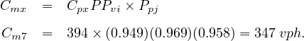
The movement capacity is found by multiplying the potential capacity by an adjustment factor. The adjustment factor is the product of the probability that each impeding movement will be blocking a subject vehicle. That is
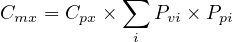 | (5) |
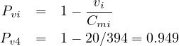
where, Cmx is the movement capacity in vph, Cpx is the potential capacity movement x in vph, Pvi is the probability that impeding vehicular movement i is not blocking the subject flow; (also referred to as the vehicular impedance factor for movement i, Ppi is the probability that impeding pedestrian movement j is not blocking the subject flow; also referred to us the pedestrian impedance factor for the movement j.
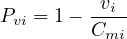
Priority 2 vehicular movements LTs from major street and RTs from minor street are not impeded by any other vehicular flow, as they represent the highest priority movements seeking gaps. They are impeded, however, by Rank 1 pedestrian movements. Priority 3 vehicular movements are impeded by Priority 2 vehicular movements and Priority l and 2 pedestrian movements seeking to use the same gaps. Priority 4 vehicular movements are impeded by Priority 2 and 3 vehicular movements, and Priority 1 and 2 pedestrian movements using the same gaps. Table. 3 lists the impeding flows for each subject movement in a four leg. Generally the rule stated the probability that impeding vehicular movement i is not blocking the subject movement is computed as
 | (6) |
where, vi is the demand flow for impeding movement i, and Cmi is the movement capacity for impeding movement i vph. Pedestrian impedance factors are computed as:
One of the impeding effects for all the movement is pedestrians movement. Both approaches of Minor-street vehicle streams must yield to pedestrian streams. Table. 3 shows that relative hierarchy between pedestrian and vehicular streams used. A factor accounting for pedestrian blockage is computed by Eqn. 7 on the basis of pedestrian volume, the pedestrian walking speed, and the lane width that is:
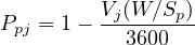 | (7) |
where, ppj is the pedestrian impedance factor for impeding pedestrian movement j, vj is the pedestrian flow rate, impeding movement j in peds/hr, w is the lane width in m, and Sp is the pedestrian walking speed in m/s.
| Vehicle Stream | Must Yield to | Impedance Factor for |
| Pedestrian Stream | Pedestrians, Pp,x | |
| V 1 | V 16 | Pp,16 |
| V 4 | V 15 | Pp,15 |
| V 7 | V 15,V 13 | (Pp,15)(Pp,13) |
| V 8 | V 15,V 16 | (Pp,15)(Pp,16) |
| V 9 | V 15,V 14 | (Pp,15)(Pp,14) |
| V 10 | V 16,V 14 | (Pp,16)(Pp,14) |
| V 11 | V 15,V 16 | (Pp,15)(Pp,16) |
| V 12 | V 16,V 13 | (Pp,16)(Pp,13) |
The capacities of individual streams (left turn, through and right turn) are calculated separately. If the streams share a common traffic lane, the capacity of the shared lane is then calculated according to the shared lane procedure. But movement capacities still represent an assumption that each minor street movement operates out of an exclusive lane. Where two or three movements share a lane its combined capacity computed as:
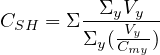 | (8) |
where, CSH is the shared lane capacity in veh/hr, V y is the flow rate, movement y sharing lane with other minor street flow, and Cmy is the movement capacity of movement y sharing lane with other minor street.
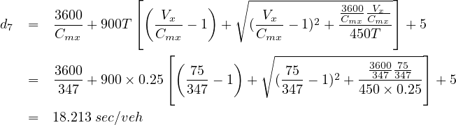
Delay is a complex measure and depends on a number of variables it is a measure of driver discomfort, frustration, fuel consumption, increased travel time etc. Total delay is the difference between the travel time actually experienced and the reference travel time that would result during base conditions, in the absence of incident, control, traffic, or geometric delay. Also, Average control delay for any particular minor movement is a function of the Capacity of the approach and The degree of saturation. The control delay per vehicle for a movement in a separate lane is given by:
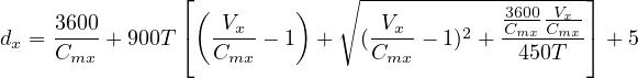 | (9) |
where, dx is the average control delay per vehicle for movement x in s/veh, Cmx is the capacity of movement or shared lane x in veh/hr, T is the analysis period h (15 min=0.25 h), and V x is the demand flow rate, movement or shared lane x in veh/hr.
Four measures are used to describe the performance of TWSC intersections: control delay, delay to major street through vehicles, queue length, and v/c ratio. The primary measure that is used to provide an estimate of LOS is control delay. This measure can be estimated for any movement on the minor (i.e., the stop-controlled) street. By summing delay estimates for individual movements, a delay estimate for each minor street movement and minor street approach can be achieved.
For AWSC intersections, the average control delay (in seconds per vehicle) is used as the primary measure of performance. Control delay is the increased time of travel for a vehicle approaching and passing through an AWSC intersection, compared with a free flow vehicle if it were not required to slow or stop at the intersection. According to the performance measure of the TWSC intersection, LOS of the minor-street left turn operates at level of service C approaches to B.
| Level of Service | Control delays(s/veh) |
| A | 0-10 |
| B | > 10-15 |
| C | > 15-25 |
| D | > 25-35 |
| E | > 35-50 |
| F | > 50 |
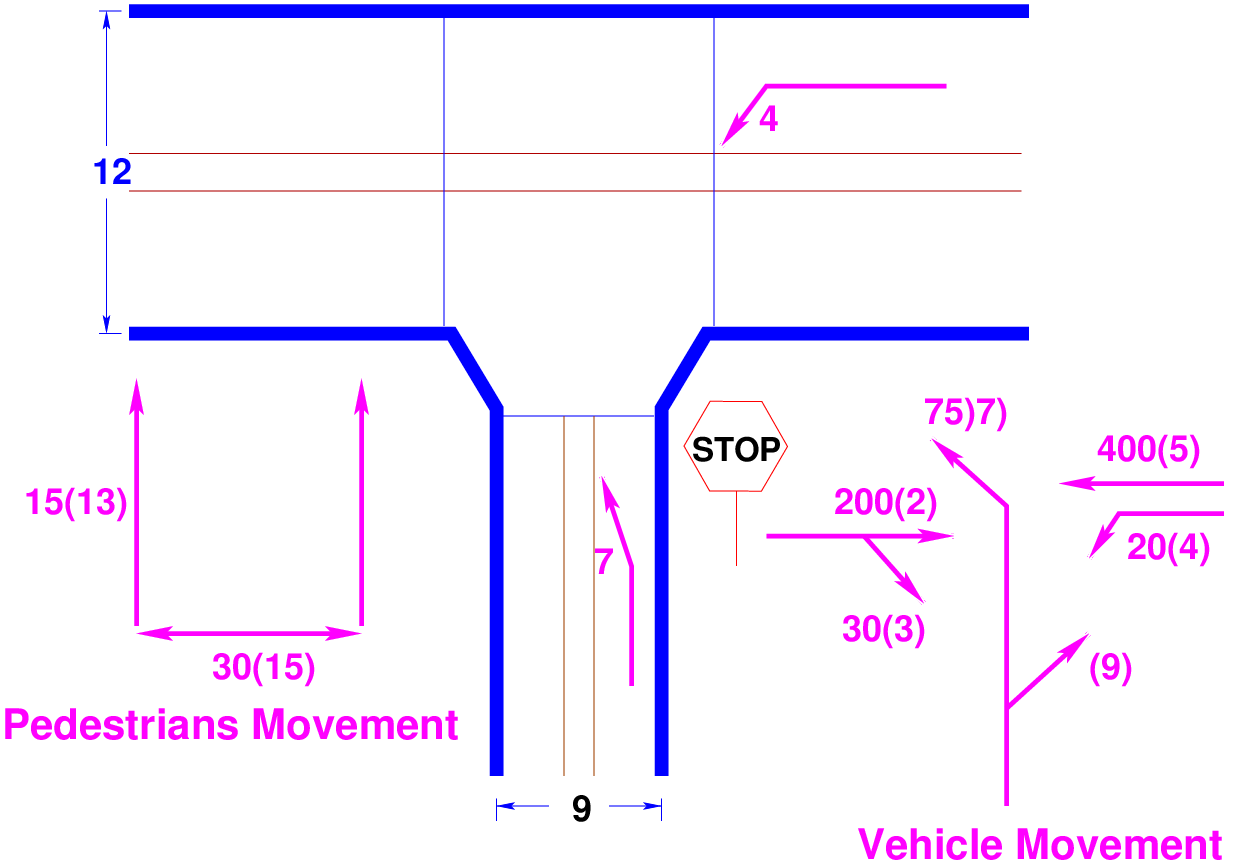
For a three legged intersection given in figure 7 determine the control delay and level of service for movement 7. The total volume of both pedestrian and vehicular traffic at each movement is given in the figure itself. Following data is also given:
![[ ]
vj × w-
Ppi = 1- ------Sp-
3600[ ]
P 13 = 1- 15-×--61.2-= 1 - 0.0417 = 0.958
p 360[0 ]
30-×--4.1.52-
Pp15 = 1- 3600 = 1 - 0.03125 = 0.969.](web11x.png)
This chapter focuses on theoretical analysis of capacity at uncontrolled intersections. First the gap acceptance theory and follow time was described; including conflict volume determination through the hierarchy of priorities for two ways stop controlled intersection. Second, after determining the potential capacity using the computed value and then prepare an adjustment for this capacity. Finally, computation of the delay to determine the level of service (LOS) of the given intersection is also described.
| Gap (sec) | Accepted gaps | Rejected gaps |
| 0.0 | 0 | 208 |
| 0.5 | 0 | 208 |
| 1.0 | 0 | 193 |
| 1.5 | 1 | 135 |
| 2.0 | 10 | 84 |
| 2.5 | 26 | 55 |
| 3.0 | 45 | 30 |
| 3.5 | 67 | 15 |
| 4.0 | 86 | 9 |
| 4.5 | 106 | 8 |
| 5.0 | 122 | 4 |
| 5.5 | 140 | 1 |
| 9.5 | 227 | 0 |
I wish to thank several of my students and staff of NPTEL for their contribution in this lecture. I wish to thank specially my student Mr. Birara Tekeste for his assistance in developing the lecture note, and my staff Ms. Reeba in typesetting the materials. I also appreciate your constructive feedback which may be sent to tvm@civil.iitb.ac.in
Prof. Tom V. Mathew
Department of Civil Engineering
Indian Institute of Technology Bombay, India
_________________________________________________________________________
Wednesday 27 September 2023 11:05:50 PM IST