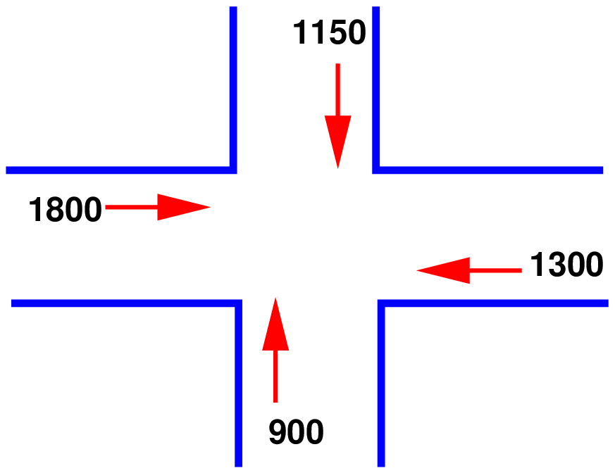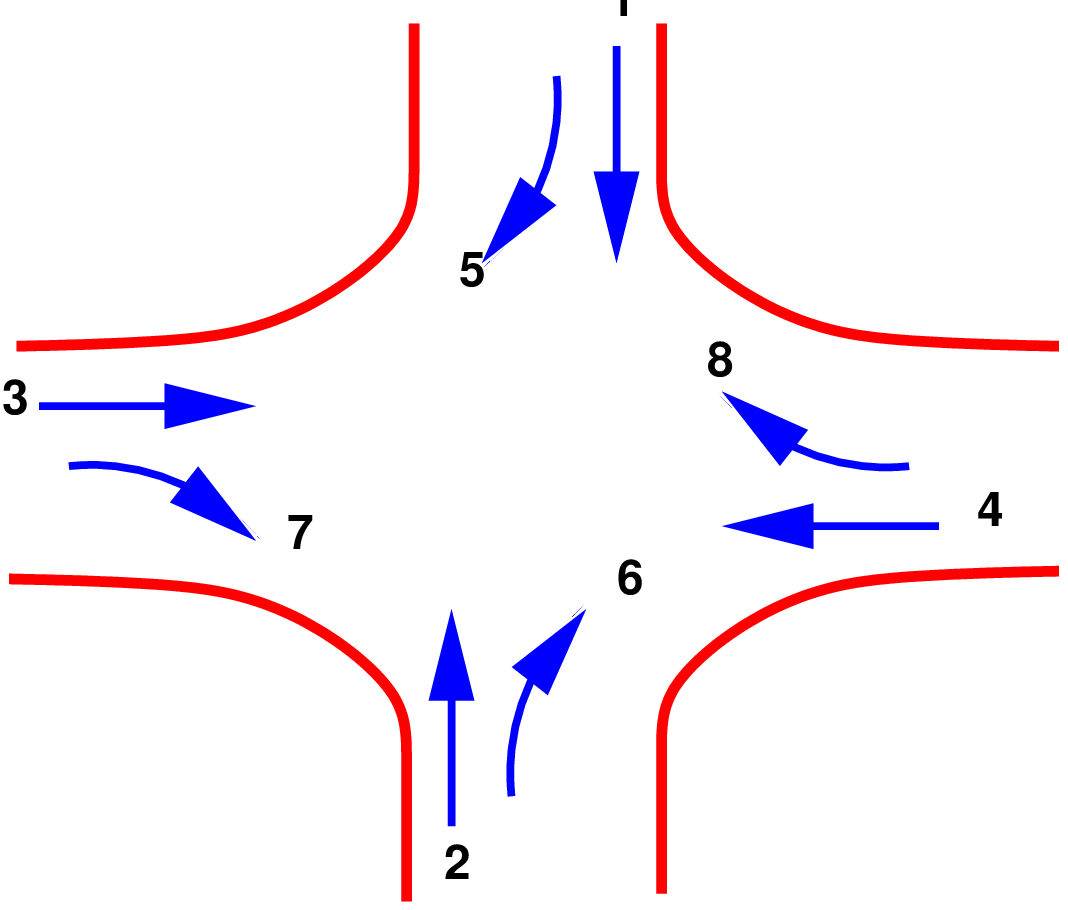
Figure 1: Four legged intersection
Traffic signals are one of the most effective and flexible active control of traffic and is widely used in several cities world wide. The conflicts arising from movements of traffic in different directions is addressed by time sharing principle. The advantages of traffic signal includes an orderly movement of traffic, an increased capacity of the intersection and requires only simple geometric design. However, the disadvantages of the signalized intersection are large stopped delays, and complexity in the design and implementation. Although the overall delay may be lesser than a rotary for a high volume, a user may experience relatively high stopped delay. This chapter discuss various design principles of traffic signal such as phase design, cycle length design, and green splitting. The concept of saturation flow, capacity, and lost times are also presented. First, some definitions and notations are given followed by various steps in design starting from phase design.
A number of definitions and notations need to be understood in signal design. They are discussed below:
The signal design procedure involves six major steps. They include: (1) phase design, (2) determination of amber time and clearance time, (3) determination of cycle length, (4) apportioning of green time, (5) pedestrian crossing requirements, and (6) performance evaluation of the design obtained in the previous steps. The objective of phase design is to separate the conflicting movements in an intersection into various phases, so that movements in a phase should have no conflicts. If all the movements are to be separated with no conflicts, then a large number of phases are required. In such a situation, the objective is to design phases with minimum conflicts or with less severe conflicts.
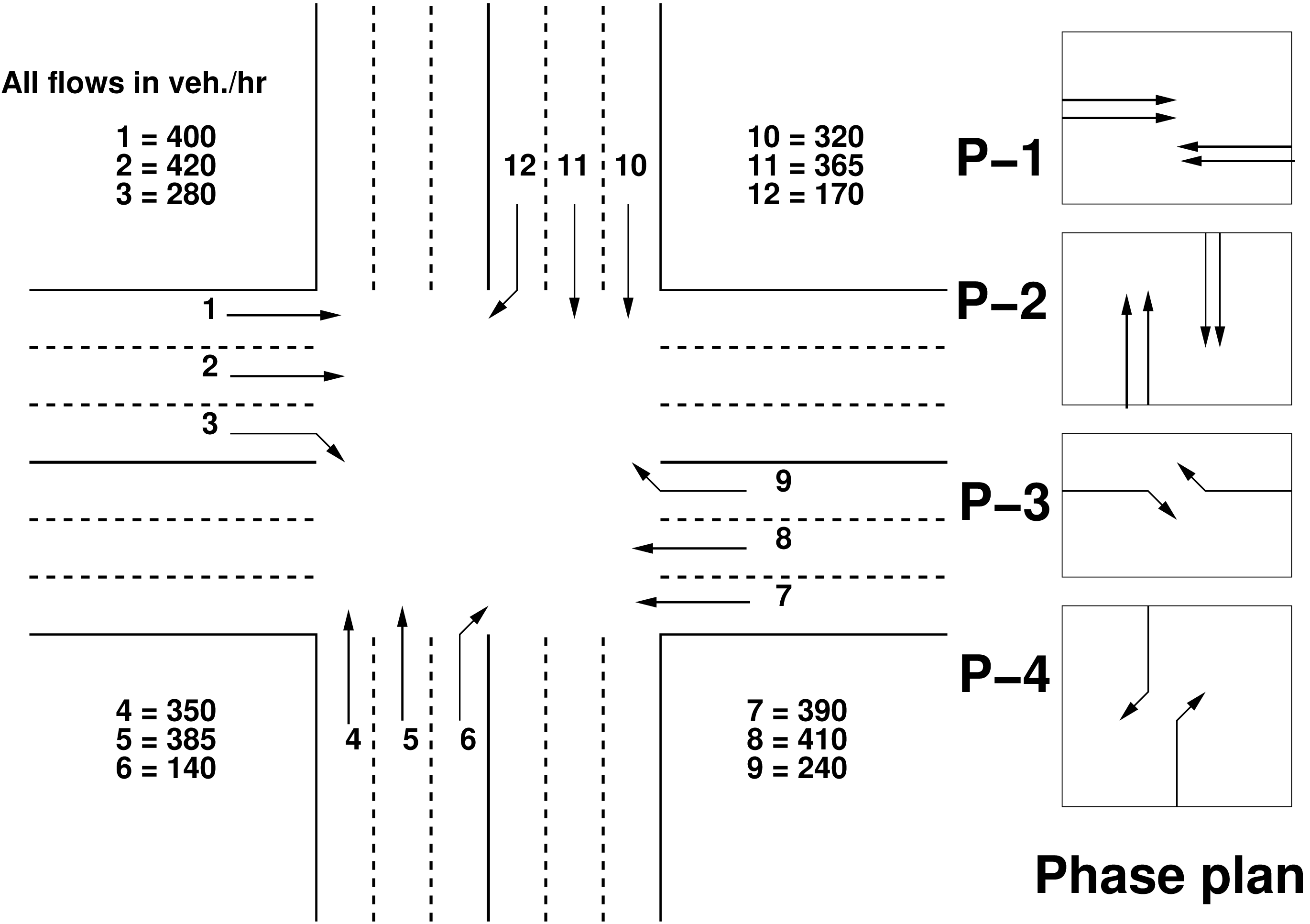
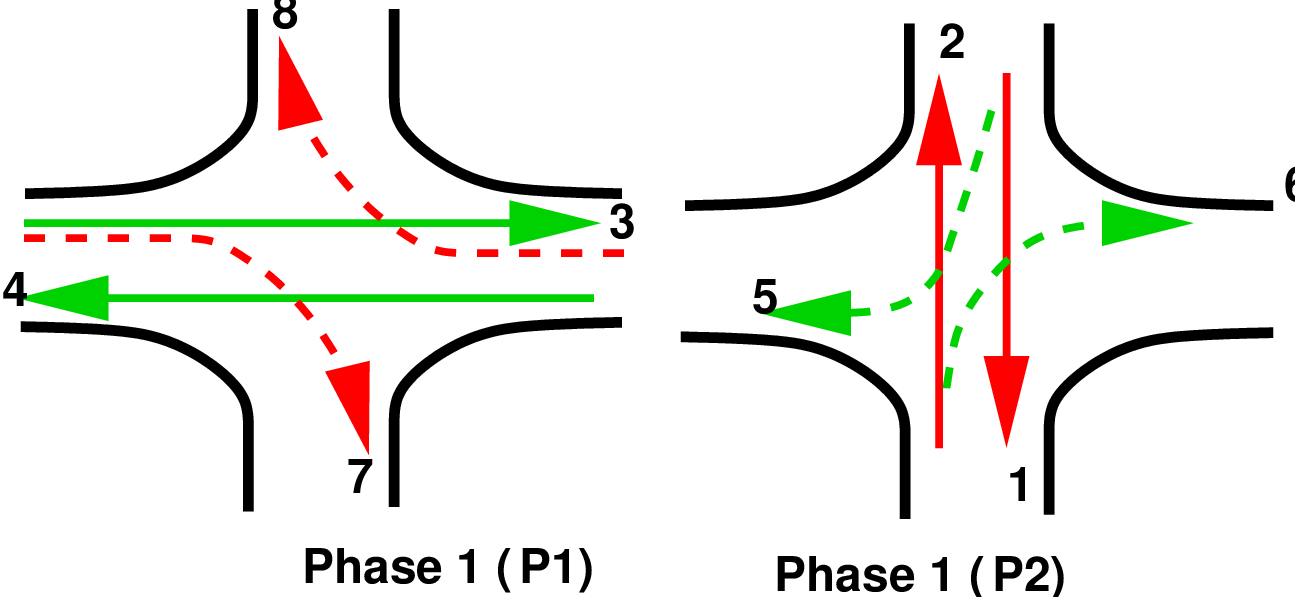
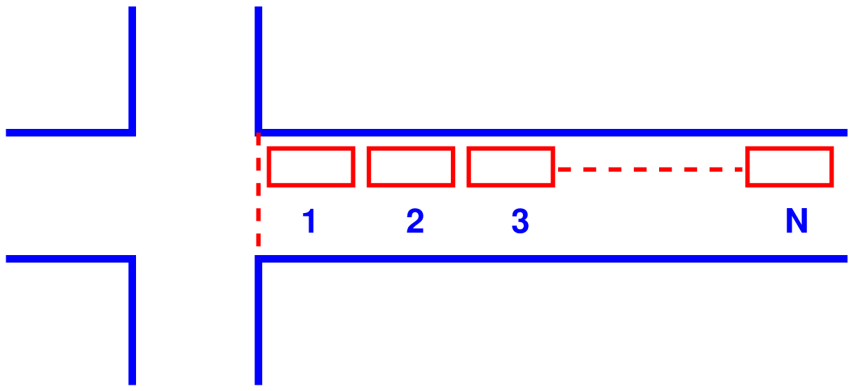
There is no precise methodology for the design of phases. This is often guided by the geometry of the intersection, the flow pattern especially the turning movements, and the relative magnitudes of flow. Therefore, a trial and error procedure is often adopted. However, phase design is very important because it affects the further design steps. Further, it is easier to change the cycle time and green time when flow pattern changes, where as a drastic change in the flow pattern may cause considerable confusion to the drivers. To illustrate various phase plan options, consider a four legged intersection with through traffic and right turns. Left turn is ignored. See Figure 1.
The first issue is to decide how many phases are required. It is possible to have two, three, four or even more number of phases.
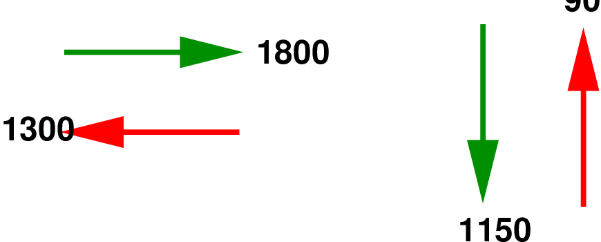
Two phase system is usually adopted if through traffic is significant compared to the turning movements. For example in Figure 2, non-conflicting through traffic 3 and 4 are grouped in a single phase and non-conflicting through traffic 1 and 2 are grouped in the second phase.
However, in the first phase flow 7 and 8 offer some conflicts and are called permitted right turns. Needless to say that such phasing is possible only if the turning movements are relatively low. On the other hand, if the turning movements are significant, then a four phase system is usually adopted.
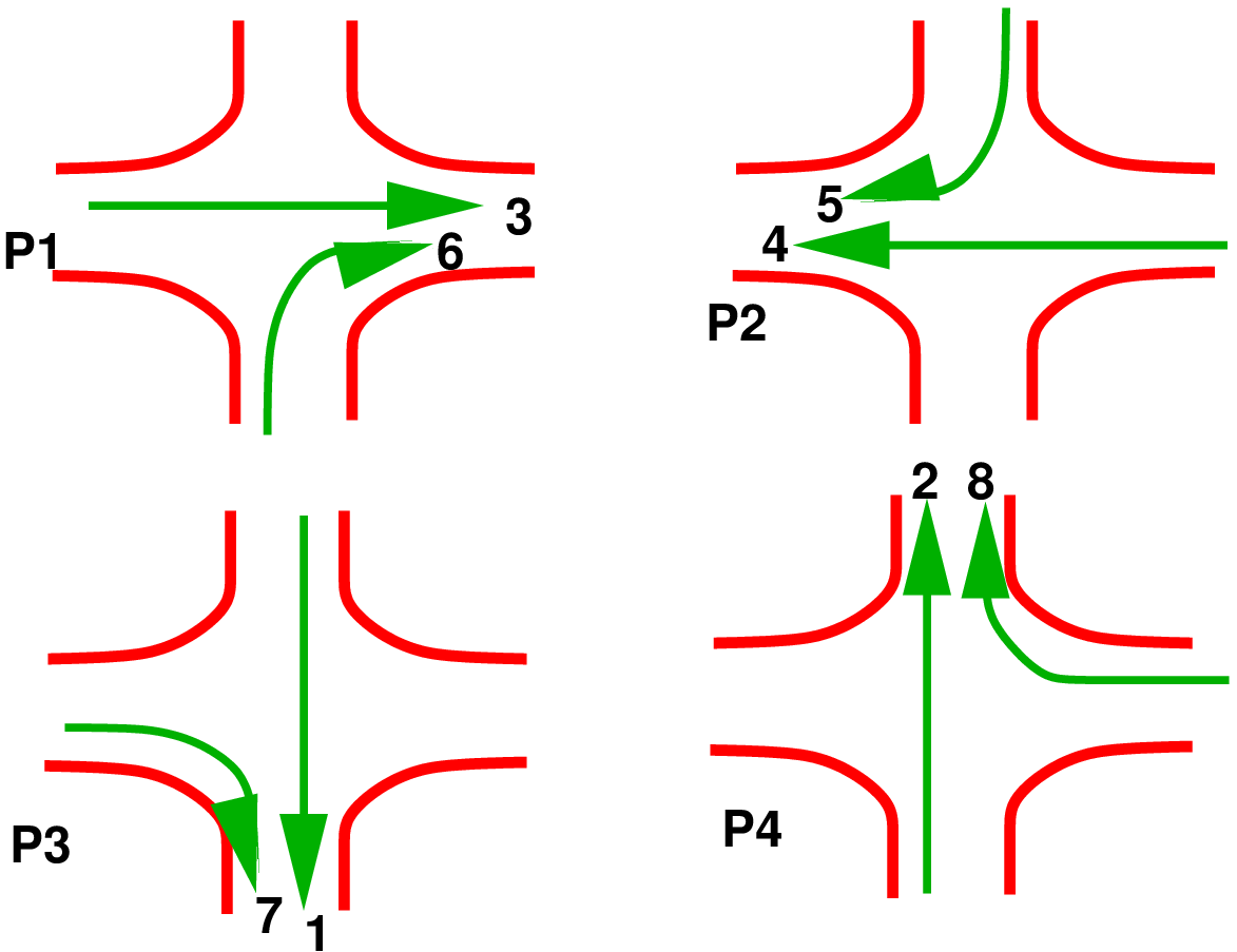
There are at least three possible phasing options. For example, Figure 3 shows the most simple and trivial phase plan.
where, flow from each approach is put into a single phase avoiding all conflicts. This type of phase plan is ideally suited in urban areas where the turning movements are comparable with through movements and when through traffic and turning traffic need to share same lane. This phase plan could be very inefficient when turning movements are relatively low.
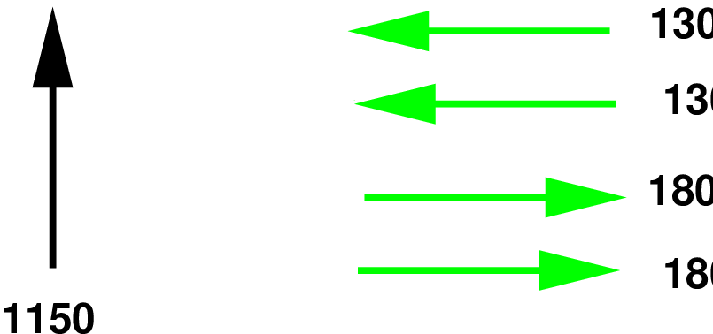
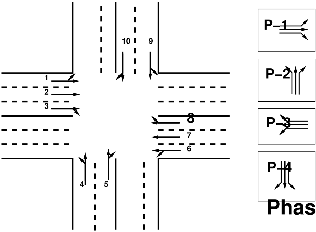
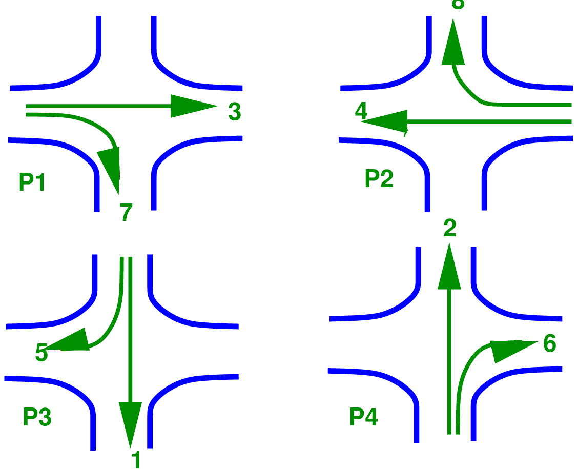
Figure 4 shows a second possible phase plan option where opposing through traffic are put into same phase.
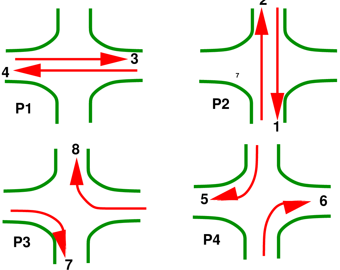
The non-conflicting right turn flows 7 and 8 are grouped into a third phase. Similarly flows 5 and 6 are grouped into fourth phase. This type of phasing is very efficient when the intersection geometry permits to have at least one lane for each movement, and the through traffic volume is significantly high. Figure 5 shows yet another phase plan. However, this is rarely used in practice.
There are five phase signals, six phase signals etc. They are normally provided if the intersection control is adaptive, that is, the signal phases and timing adapt to the real time traffic conditions.
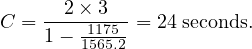
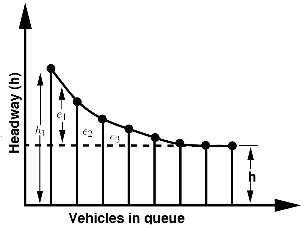
Cycle time is the time taken by a signal to complete one full cycle of iterations. i.e. one complete rotation through all signal indications. It is denoted by C. The way in which the vehicles depart from an intersection when the green signal is initiated will be discussed now. Figure 6 illustrates a group of N vehicles at a signalized intersection, waiting for the green signal.
As the signal is initiated, the time interval between two vehicles, referred as headway, crossing the curb line is noted. The first headway is the time interval between the initiation of the green signal and the instant vehicle crossing the curb line. The second headway is the time interval between the first and the second vehicle crossing the curb line. Successive headways are then plotted as in Figure 7.
The first headway will be relatively longer since it includes the reaction time of the driver and the time necessary to accelerate. The second headway will be comparatively lower because the second driver can overlap his/her reaction time with that of the first driver’s. After few vehicles, the headway will become constant. This constant headway which characterizes all headways beginning with the fourth or fifth vehicle, is defined as the saturation headway, and is denoted as h. This is the headway that can be achieved by a stable moving platoon of vehicles passing through a green indication. If every vehicles require h seconds of green time, and if the signal were always green, then s vehicles per hour would pass the intersection. Therefore,
 | (1) |
where s is the saturation flow rate in vehicles per hour of green time per lane, h is the saturation headway in seconds. As noted earlier, the headway will be more than h particularly for the first few vehicles. The difference between the actual headway and h for the ith vehicle and is denoted as ei shown in Figure 7. These differences for the first few vehicles can be added to get start up lost time, Li which is given by,
 | (2) |
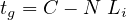
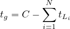
The green time required to clear N vehicles can be found out as,
 | (3) |
where T is the time required to clear N vehicles through signal, Li is the start-up lost time, and h is the saturation headway in seconds.
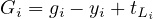
Effective green time is the actual time available for the vehicles to cross the intersection. It is the sum of actual green time (Gi) plus the yellow minus the applicable lost times. Thus effective green time can be written as,
 | (4) |
The ratio of effective green time to the cycle length ( )is defined as green ratio. We know that
saturation flow rate is the number of vehicles that can be moved in one lane in one hour
assuming the signal to be green always. Then the capacity of a lane can be computed
as,
)is defined as green ratio. We know that
saturation flow rate is the number of vehicles that can be moved in one lane in one hour
assuming the signal to be green always. Then the capacity of a lane can be computed
as,
 | (5) |
where ci is the capacity of lane in vehicle per hour, si is the saturation flow rate in vehicle per hour per lane, C is the cycle time in seconds.
Let the cycle time of an intersection is 60 seconds, the green time for a phase is 27 seconds, and the corresponding yellow time is 4 seconds. If the saturation headway is 2.4 seconds per vehicle, and the start-up lost time is 3 seconds per phase, find the capacity of the movement per lane?
 =
=  = 1500 veh per hr.
 = 700 veh per hr per lane.
During any green signal phase, several lanes on one or more approaches are permitted to move. One of these will have the most intense traffic. Thus it requires more time than any other lane moving at the same time. If sufficient time is allocated for this lane, then all other lanes will also be well accommodated. There will be one and only one critical lane in each signal phase. The volume of this critical lane is called critical lane volume.
The cycle length or cycle time is the time taken for complete indication of signals in a cycle. Fixing the cycle length is one of the crucial steps involved in signal design. An expression for computing the cycle length can be derived as follows.
 .
.
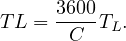
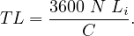
 . Now, the signal time shold be designed in
such a way that this number should be the critical intersection volume per hour is V c.
That is,
. Now, the signal time shold be designed in
such a way that this number should be the critical intersection volume per hour is V c.
That is,

 | (8) |
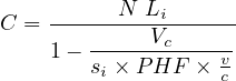
Highway capacity manual (HCM) has given an equation for determining the cycle length which is a slight modification of the above equation (setting Xc = PHF × v∕c and rewriting the equation). Accordingly, cycle time C is given by,
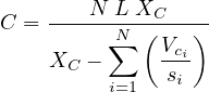 | (9) |
where N is the number of phases, L is the lost time per phase,  is the ratio of critical
volume to saturation flow for phase i, XC is the quality factor called the degree of
saturation.
is the ratio of critical
volume to saturation flow for phase i, XC is the quality factor called the degree of
saturation.
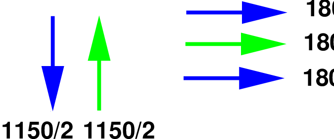
The traffic flow in an intersection is shown in the Figure 8.
Given start-up lost time is 3 seconds, saturation head way is 2.3 seconds, compute the cycle length for that intersection. Assume a two-phase signal.
Similarly critical volume for the second phase = 1800 vph. Therefore, total critical volume for the two signal phases = 1150+1800 = 2950 vph.
 = 1565.2 vph. This means, that the intersection can handle
only 1565.2 vph. However, the critical volume is 2950 vph . Hence the critical
lane volume should be reduced and one simple option is to split the major
traffic into two lanes. So the resulting phase plan is as shown in Figure 10.
= 1565.2 vph. This means, that the intersection can handle
only 1565.2 vph. However, the critical volume is 2950 vph . Hence the critical
lane volume should be reduced and one simple option is to split the major
traffic into two lanes. So the resulting phase plan is as shown in Figure 10.
 |
Green splitting or apportioning of green time is the proportioning of effective green time in each of the signal phase. The green splitting is given by,
![[ ]
---Vci--
gi = ∑N Vc × tg
i=1 i](web22x.png) | (10) |
where V ci is the critical lane volume and tg is the total effective green time available in a cycle. This will be cycle time minus the total lost time for all the phases. Therefore,
 | (11) |
where C is the cycle time in seconds, n is the number of phases, and Li is the lost time per phase. If lost time is different for different phases, then effective green time can be computed as follows:
 | (12) |
where tLi is the lost time for phase i, N is the number of phases and C is the cycle time in seconds. Actual green time can be now found out as,
 | (13) |
where Gi is the actual green time, gi is the effective green time available, yi is the amber time, and Li is the lost time for phase i.
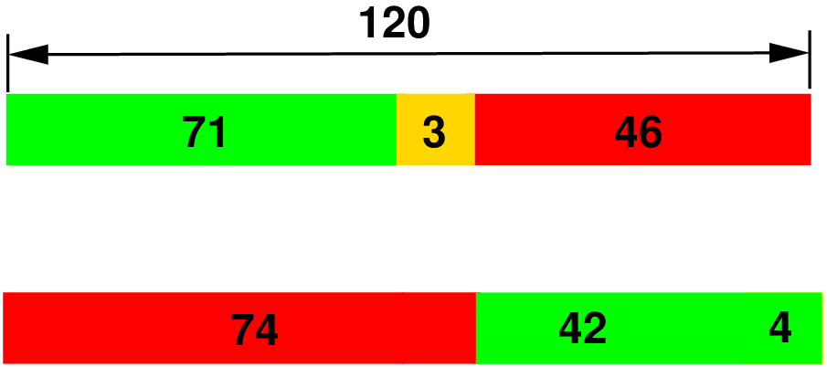
The phase diagram with flow values of an intersection with two phases is shown in Figure 12.
The lost time and yellow time for the first phase is 2.5 and 3 seconds respectively. For the second phase the lost time and yellow time are 3.5 and 4 seconds respectively. If the cycle time is 120 seconds, find the green time allocated for the two phases.
 × 114 = 71.25 seconds.
 × 114= 42.75 seconds.
Traffic signal is an aid to control traffic at intersections where other control measures fail. The signals operate by providing right of way to a certain set of movements in a cyclic order. The design procedure discussed in this chapter include phase design, interval design, determination of cycle time, computation of saturation flow, and green splitting.
I wish to thank several of my students and staff of NPTEL for their contribution in this lecture. I also appreciate your constructive feedback which may be sent to tvm@civil.iitb.ac.in
Prof. Tom V. Mathew
Department of Civil Engineering
Indian Institute of Technology Bombay, India
_________________________________________________________________________
Thursday 28 September 2023 10:46:32 AM IST
![Tg = 3600- TL
= 3600- 3600-N-Li
[ C ]
N-Li-
= 3600 1- C (6 )](web13x.png)
![V = Tg,
c h [ ]
3600 N-Li-
= h 1 - C ,
[ N Li]
= si 1 - -C--- ,
∴ C = N--LVi. (7 )
1- sci](web16x.png)