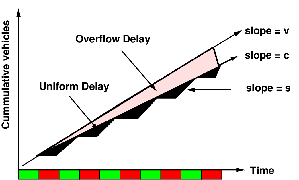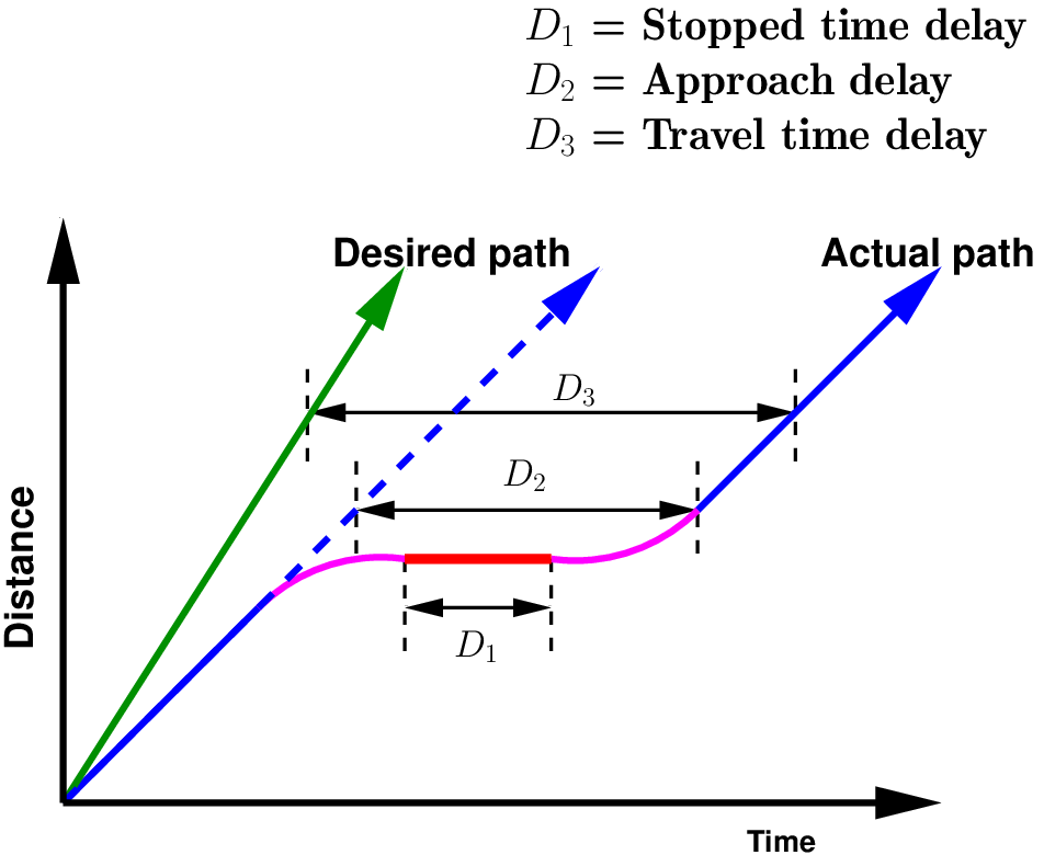
Figure 1: Illustration of various types of delay measures
Signalized intersections are the important points or nodes within a system of highways and streets. To describe some measure of effectiveness to evaluate a signalized intersection or to describe the quality of operations is a difficult task. There are a number of measures that have been used in capacity analysis and simulation, all of which quantify some aspect of experience of a driver traversing a signalized intersection. The most common measures are average delay per vehicle, average queue length, and number of stops. Delay is a measure that most directly relates driver’s experience and it is measure of excess time consumed in traversing the intersection. Length of queue at any time is a useful measure, and is critical in determining when a given intersection will begin to impede the discharge from an adjacent upstream intersection. Number of stops made is an important input parameter, especially in air quality models. Among these three, delay is the most frequently used measure of effectiveness for signalized intersections for it is directly perceived by a driver. The estimation of delay is complex due to random arrival of vehicles, lost time due to stopping of vehicles, over saturated flow conditions etc. This chapter looks are some important models to estimate delays.
The most common measure of operational quality is delay, although queue length is often used as a secondary measure. While it is possible to measure delay in the field, it is a difficult process, and different observers may make judgments that could yield different results. For many purposes, it is, therefore, convenient to have a predictive model for the estimate of delay. Delay, however, can be quantified in many different ways. The most frequently used forms of delay are defined as follows:
These delay measures can be quite different, depending on conditions at the signalized intersection. Fig 1 shows the differences among stopped time, approach and travel time delay for single vehicle traversing a signalized intersection. The desired path of the vehicle is shown, as well as the actual progress of the vehicle, which includes a stop at a red signal.
Note that the desired path is the path when vehicles travel with their preferred speed and the actual path is the path accounting for decreased speed, stops and acceleration and deceleration.
Stopped-time delay is defined as the time a vehicle is stopped in queue while waiting to pass through the intersection. It begins when the vehicle is fully stopped and ends when the vehicle begins to accelerate. Average stopped-time delay is the average for all vehicles during a specified time period.
Approach delay includes stopped-time delay but adds the time loss due to deceleration from the approach speed to a stop and the time loss due to re-acceleration back to the desired speed. It is found by extending the velocity slope of the approaching vehicle as if no signal existed. Approach delay is the horizontal (time) difference between the hypothetical extension of the approaching velocity slope and the departure slope after full acceleration is achieved. Average approach delay is the average for all vehicles during a specified time period.
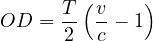
It is the difference between the driver’s expected travel time through the intersection (or any roadway segment) and the actual time taken. To find the desired travel time to traverse an intersection is very difficult. So this delay concept is is rarely used except in some planning studies.
Time-in-queue delay is the total time from a vehicle joining an intersection queue to its discharge across the STOP line on departure. Average time-in-queue delay is the average for all vehicles during a specified time period. Time-in-queue delay cannot be effectively shown using one vehicle, as it involves joining and departing a queue of several vehicles.
Control delay is the delay caused by a control device, either a traffic signal or a STOP-sign. It is approximately equal to time-in-queue delay plus the acceleration-deceleration delay component. Delay measures can be stated for a single vehicle, as an average for all vehicles over a specified time period, or as an aggregate total value for all vehicles over a specified time period. Aggregate delay is measured in total vehicle-seconds, vehicle-minutes, or vehicle-hours for all vehicles in the specified time interval. Average individual delay is generally stated in terms of seconds per vehicle for a specified time interval.
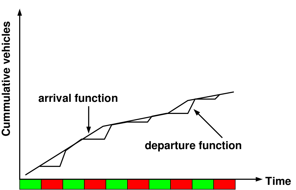
In analytic models for predicting delay, there are three distinct components of delay, namely, uniform delay, random delay, and overflow delay. Before, explaining these, first a delay representation diagram is useful for illustrating these components.
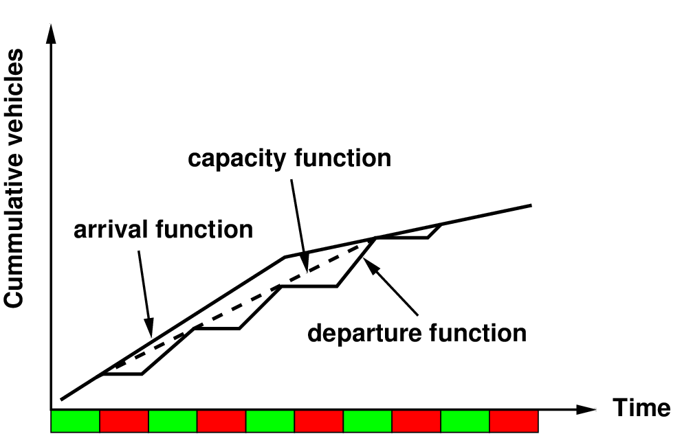
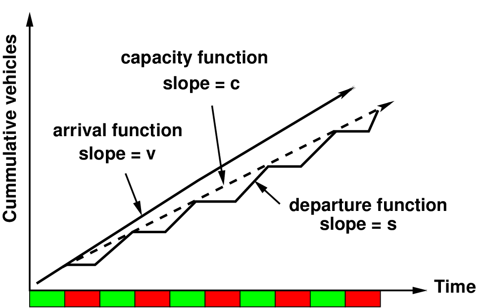
All analytic models of delay begin with a plot of cumulative vehicles arriving and departing vs. time at a given signal location. Figure 2 shows a plot of total vehicle vs time. Two curves are shown: a plot of arriving vehicles and a plot of departing vehicles. The time axis is divided into periods of effective green and effective red. Vehicles are assumed to arrive at a uniform rate of flow (v vehicles per unit time). This is shown by the constant slope of the arrival curve. Uniform arrivals assume that the inter-vehicle arrival time between vehicles is a constant. Assuming no preexisting queue, arriving vehicles depart instantaneously when the signal is green (ie., the departure curve is same as the arrival curve). When the red phase begins, vehicles begin to queue, as none are being discharged. Thus, the departure curve is parallel to the x-axis during the red interval. When the next effective green begins, vehicles queued during the red interval depart from the intersection, at a rate called saturation flow rate (s vehicle per unit time). For stable operations, depicted here, the departure curve catches up with the arrival curve before the next red interval begins (i.e., there is no residual queue left at the end of the effective green).
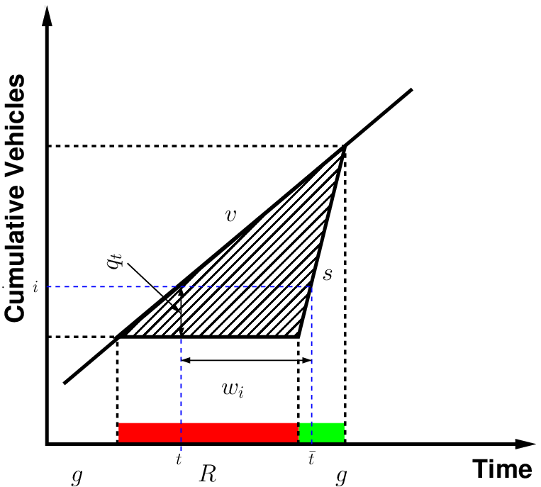
In this simple model:
Uniform delay is the delay based on an assumption of uniform arrivals and stable flow with no individual cycle failures. Figure 3, shows stable flow throughout the period depicted. No signal cycle fails here, i.e., no vehicles are forced to wait for more than one green phase to be discharged. During every green phase, the departure function catches up with the arrival function. Total aggregate delay during this period is the total of all the triangular areas between the arrival and departure curves. This type of delay is known as Uniform delay where uniform vehicle arrival is assumed.
Random delay is the additional delay, above and beyond uniform delay, because flow is randomly distributed rather than uniform at isolated intersections. In Figure 4 some of the signal phases fail. At the end of the second and third green intervals, some vehicles are not served (i.e., they must wait for a second green interval to depart the intersection). By the time the entire period ends, however, the departure function has caught up with the arrival function and there is no residual queue left unserved. This case represents a situation in which the overall period of analysis is stable (ie.,total demand does not exceed total capacity). Individual cycle failures within the period, however, have occurred. For these periods, there is a second component of delay in addition to uniform delay. It consists of the area between the arrival function and the dashed line, which represents the capacity of the intersection to discharge vehicles, and has the slope c. This type of delay is referred to as Random delay.
Overflow delay is the additional delay that occurs when the capacity of an individual phase or series of phases is less than the demand or arrival flow rate. Figure 5 shows the worst possible case, every green interval fails for a significant period of time, and the residual, or unserved, queue of vehicles continues to grow throughout the analysis period. In this case, the overflow delay component grows over time, quickly dwarfing the uniform delay component. The latter case illustrates an important practical operational characteristic. When demand exceeds capacity (v∕c > 1.0), the delay depends upon the length of time that the condition exists. In Figure 4, the condition exists for only two phases. Thus, the queue and the resulting overflow delay is limited. In Figure 5, the condition exists for a long time, and the delay continues to grow throughout the over-saturated period. This type of delay is referred to as Overflow delay
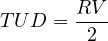
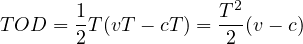
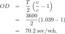
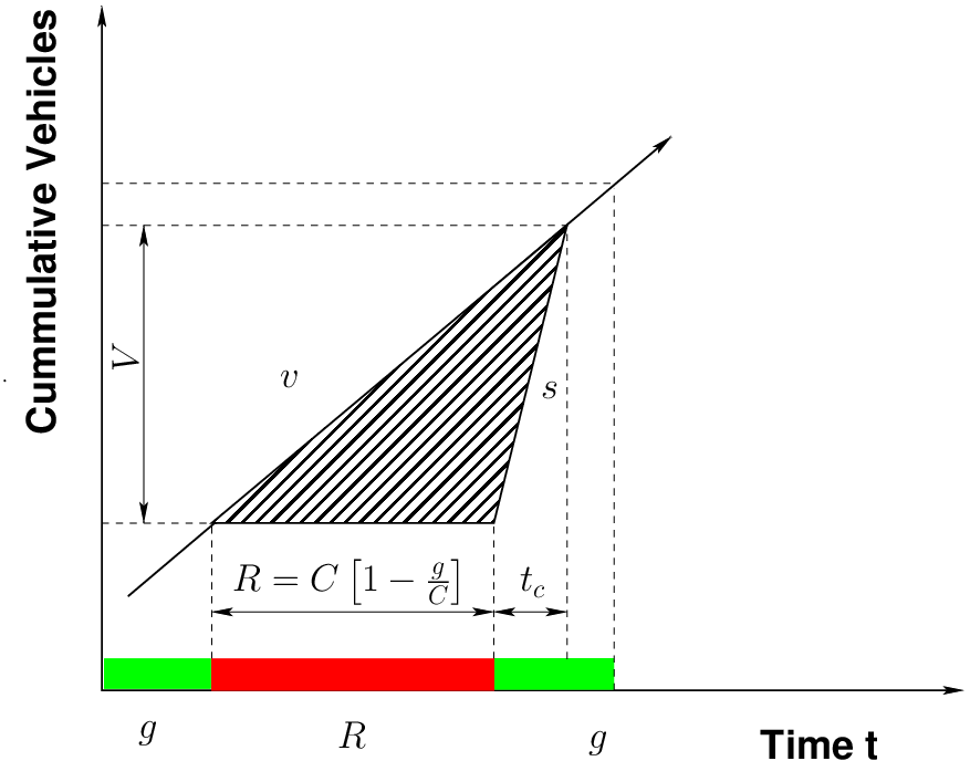
Model is explained based on the assumptions of stable flow and a simple uniform arrival function. As explained in the above section, aggregate delay can be estimated as the area between the arrival and departure curves. Thus, Webster’s model for uniform delay is the area of the triangle formed by the arrival and departure functions. From Figure 6 the area of the aggregate delay triangle is simply one-half the base times the height. Hence, the total uniform delay (TUD) is given as:
 | (1) |
where, R is the duration of red, V is the number of vehicles arriving during the time interval R + tc. Length of red phase is given as the proportion of the cycle length which is not green, or:
 | (2) |
The height of the triangle is found by setting the number of vehicles arriving during the time (R + tc) equal to the number of vehicles departing in time tc, or:
 | (3) |
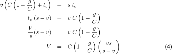
Substituting Equation 2 for R in Equation 3 and solving for tc and then for V gives,
Substituting Equation 2 and Equation 4 in Equation 1 gives:![RV
T UD = ---
2[ ( )]2( )
= 1 C 1- -g -vs--
2 C s- v](web4x.png)
 | (6) |
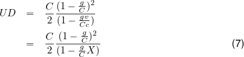
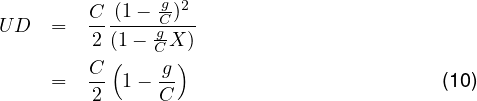
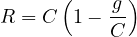
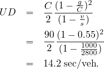
So, the relation for uniform delay changes to,
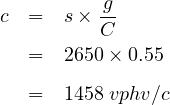
where, UD is the uniform delay (sec/vehicle) C is the cycle length (sec), c is the capacity, v is the vehicle arrival rate, s is the saturation flow rate or departing rate of vehicles, X is the v/c ratio or degree of saturation (ratio of the demand flow rate to saturation flow rate), and g∕C is the effective green ratio for the approach.Consider the following situation: An intersection approach has an approach flow rate of 1,000 vph, a saturation flow rate of 2,800 vph, a cycle length of 90 s, and effective green ratio of 0.44 for the approach. What average delay per vehicle is expected under these conditions?
Solution: First, the capacity and v/c ratio for the intersection approach must be computed. Given, s=2800 vphg and g/C=0.55. Hence,
The uniform delay model assumes that arrivals are uniform and that no signal phases fail (i.e., that arrival flow is less than capacity during every signal cycle of the analysis period). At isolated intersections, vehicle arrivals are more likely to be random. A number of stochastic models have been developed for this case, including those by Newell, Miller and Webster. These models generally assume that arrivals are Poisson distributed, with an underlying average rate of v vehicles per unit time. The models account for random arrivals and the fact that some individual cycles within a demand period with v∕c < 1.0 could fail due to this randomness. This additional delay is often referred to as Random delay. The most frequently used model for random delay is Webster’s formulation:
 | (8) |
where, RD is the average random delay per vehicle, s/veh, and X is the degree of saturation (v/c ratio). Webster found that the above delay formula overestimate delay and hence he proposed that total delay is the sum of uniform delay and random delay multiplied by a constant for agreement with field observed values. Accordingly, the total delay is given as:
 | (9) |
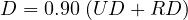
Model is explained based on the assumption that arrival function is uniform. In this model a new term called over saturation is used to describe the extended time periods during which arrival vehicles exceeds the capacity of the intersection approach to the discharged vehicles. In such cases queue grows and there will be overflow delay in addition to the uniform delay. Figure 7 illustrates a time period for which v∕c > 1.0.
During the period of over-saturation delay consists of both uniform delay (in the triangles between the capacity and departure curves) and overflow delay (in the triangle between arrival and capacity curves). As the maximum value of X is 1.0 for uniform delay, it can be simplified as,
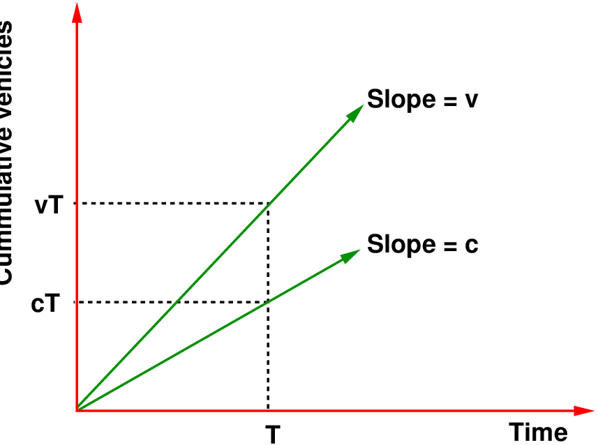
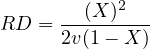
From Figure 8 total overflow delay can be estimated as,
 | (11) |
where, TOD is the total or aggregate overflow delay (in veh-secs), and T is the analysis period in seconds. Average delay is obtained by dividing the aggregate delay by the number of vehicles discharged with in the time T which is cT.
 | (12) |
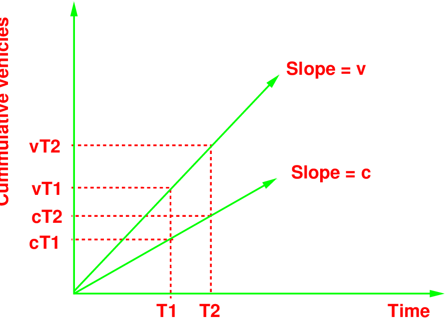
The delay includes only the delay accrued by vehicles through time T, and excludes additional delay that vehicles still stuck in the queue will experience after time T. The above said delay equation is time dependent i.e., the longer the period of over-saturation exists, the larger delay becomes. A model for average overflow delay during a time period T1 through T2 may be developed, as illustrated in Figure 9 Note that the delay area formed is a trapezoid, not a triangle. The resulting model for average delay per vehicle during the time period T1 through T2 is:
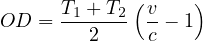 | (13) |
Formulation predicts the average delay per vehicle that occurs during the specified interval, T1 through T2. Thus, delays to vehicles arriving before time T1 but discharging after T1 are included only to the extent of their delay within the specified times, not any delay they may have experienced in queue before T1. Similarly, vehicles discharging after T2 are not included in the formulation.
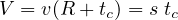
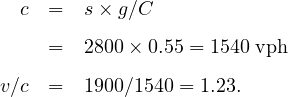
Consider the following situation: An intersection approach has an approach flow rate of 1,900 vph, a saturation flow rate of 2,800 vphg, a cycle length of 90s, and effective green ratio for the approach 0.55. What average delay per vehicle is expected under these conditions?
Solution: To begin, the capacity and v/c ratio for the intersection approach must be computed. This will determine what model(s) are most appropriate for application in this case: Given, s=2800 vphg, g/C=0.55, and v =1900 vph.
![D = UD + OD
C ( g )
UD = -2 1- C-
= 0.5× 90[1 - 0.55]
= 20.3
T ( v )
OD = -2 c - 1
3600
= --2-(1.23- 1)
= 414
D = 20.3+ 414
= 434.3 sec∕veh](web17x.png)
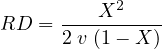
As explained earlier random and overflow delay is given as, Random delay,
 | (14) |
Overflow delay,
 | (15) |
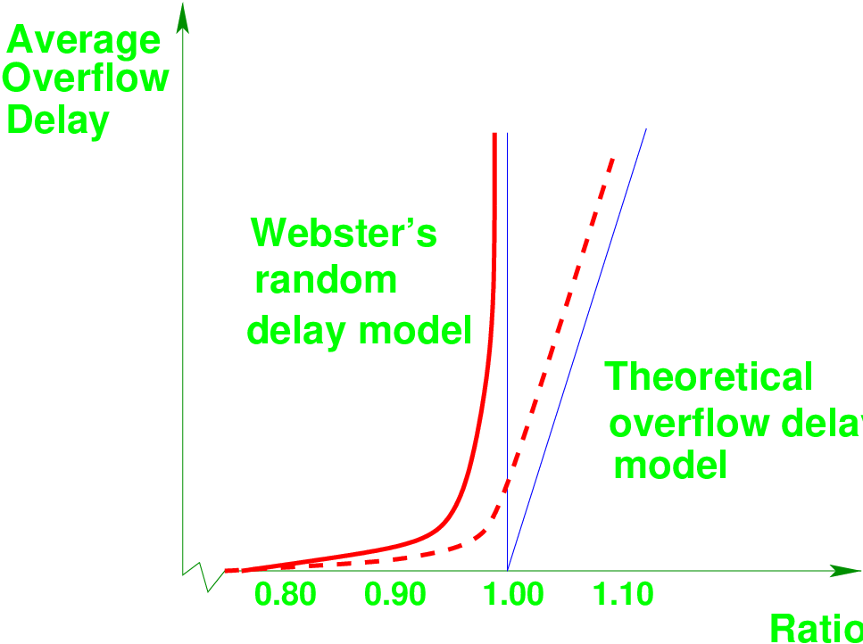
The inconsistency occurs when the X is in the vicinity of 1.0. When X < 1.0 random delay model is used. As the Webster’s random delay contains 1-X term in the denominator, when X approaches to 1.0 random delay increases asymptotically to infinite value. When X > 1.0 overflow delay model is used. Overflow delay contains 1 - X term in the numerator, when X approaches to 1.0 overflow becomes zero and increases uniformly with increasing value of X. Both models are not accurate in the vicinity of X = 1.0. Delay does not become infinite at X = 1.0. There is no true overflow at X = 1.0, although individual cycle failures due to random arrivals do occur. Similarly, the overflow model, with overflow delay of zero seconds per vehicle at X = 1.0 is also unrealistic. The additional delay of individual cycle failures due to the randomness of arrivals is not reflected in this model. Most studies show that uniform delay model holds well in the range X ≤ 0.85. In this range true value of random delay is minimum and there is no overflow delay. Also overflow delay model holds well when X ≥ 1.15. The inconsistency occurs in the range 0.85 ≤ X ≤ 1.15; here both the models are not accurate. Much of the more recent work in delay modeling involves attempts to bridge this gap, creating a model that closely follows the uniform delay model at low X ratios, and approaches the theoretical overflow delay model at high X ratios, producing ”reasonable” delay estimates in between. Figure 10 illustrates this as the dashed line.
The most commonly used model for intersection delay is to fit models that works well under all v/c ratios. Few of them will be discussed here.
To address the above said problem Akcelik proposed a delay model and is used in the Australian Road Research Board’s signalized intersection. In his delay model, overflow component is given by,
![[ ∘ --------------------]
cT- 2 12(X--- X0-)
OD = 4 (X - 1)+ (X - 1) + cT](web20x.png)
 | (16) |
where, T is the analysis period, h, X is the v/c ratio, c is the capacity, veh/hour, s is the saturation flow rate, veh/sg (vehicles per second of green) and g is the effective green time, sec
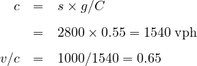
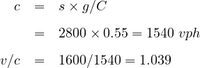
Consider the following situation: An intersection approach has an approach flow rate of 1,600 vph, a saturation flow rate of 2,800 vphg, a cycle length of 90s, and a g/C ratio of 0.55. What average delay per vehicle is expected under these conditions?
Solution: To begin, the capacity and v/c ratio for the intersection approach must be computed. This will determine what model(s) are most appropriate for application in this case: Given, s =2800 vphg; g/C=0.55; v =1600 vph
![UD = C-(1- -g)
2 C
= 0.5× 90[1 - 0.55]
= 20.3 sec∕veh.](web23x.png)
![[ ∘ --------------------]
OD = cT- (X - 1)+ (X - 1)2 + 12(X----X0)
4 cT
g = 0.55× 90 = 49.5 sec
s = 2800∕3600 = 0.778 veh∕sec
0.778-×-49.5-
X0 = 0.67+ 600 = 0.734
X - 1 = 1.039- 1 ≈ 0.4
[ ∘---------------------]
OD = 1540 0.4 + 0.42 + 12(1.039---0.734)
4 1540
= 39.1 sec∕veh](web24x.png)
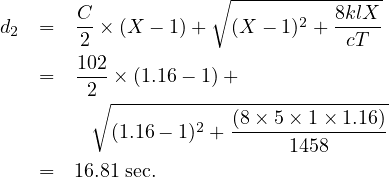
The delay model incorporated into the HCM 2000 includes the uniform delay model, a version of Akcelik’s overflow delay model, and a term covering delay from an existing or residual queue at the beginning of the analysis period. The delay is given as,
![d = d1 P F + d2 + d3
c (1 - g)2
d1 = 2 × 1--[min(1c,X-)(g)]
[ ∘-c-------------]
2 8klX-
d2 = 900T (X - 1) + (X - 1) + cT
( )
PF = -(1---P)-- × fp
(1 - (g∕c)](web26x.png)
Consider the following situation: An intersection approach has an approach flow rate of 1,400 vph, a saturation flow rate of 2,650 vphg, a cycle length of 102 s, and effective green ratio for the approach 0.55. Assume Progression Adjustment Factor 1.25 and delay due to pre-existing queue, 12 sec/veh. What control delay sec per vehicle is expected under these conditions?
Solution: Saturation flow rate =2650 vphg , g/C=0.55, Approach flow rate v=1700 vph, Cycle length C=102 sec, delay due to pre-existing queue =12 sec/veh and Progression Adjustment Factor PF=1.25. The capacity is given as:
![g-2
d1 = C-----(1---C)--g--
2[1- min (X, 1)(c)]
102 ----(1--1.16)2-----
= 2 [1 - min (1.16,1)(.55)] = 22.95](web28x.png)
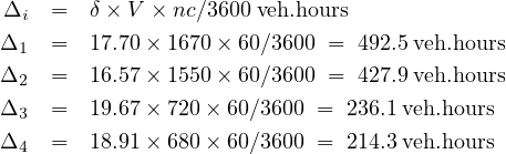
In this chapter measure of effectiveness at signalized intersection are explained in terms of delay. Different forms of delay like stopped time delay, approach delay, travel delay, time-in-queue delay and control delay are explained. Types of delay like uniform delay, random delay and overflow delay are explained and corresponding delay models are also explained above. Inconsistency between delay models at v/c=1.0 is explained in the above section and the solution to the inconsistency, delay model proposed by Akcelik is explained. At last HCM 2000 delay model is also explained in this section. From the study, various form of delay occurring at the intersection is explained through different models, but the delay calculated using such models may not be accurate as the models are explained on the theoretical basis only.
![C-[1- -g]2
δ = -2[---Cv]--
1[ - s ]
602 1 - 2760-2
δ1 = -[1---835]- = 17.70 sec∕cycle
[ 1714]2
602[-1---2760]-
δ2 = 1- 1777514- = 16.57 sec∕cycle
60[ 23]2
δ3 = -2[-1---60]- = 19.67 sec∕cycle
1- 1727014-
60[1 - 23]2
δ4 = -2[----68600]- = 18.91 sec∕cycle
1- 1714](web31x.png)
| h | 2.1 | ||||
| s | 1714.3 | ||||
| xc | 0.9 | ||||
| p1 | p1 | p3 | p4 | Cum | |
| L | 2.4 | 2.4 | 2.4 | 2.4 | 9.6 |
| q1 | 300.0 | 120.0 | 180.0 | 170.0 | |
| q2 | 400.0 | 365.0 | 110.0 | 360.0 | |
| q3 | 410.0 | 185.0 | 0.0 | 0.0 | |
| q4 | 110.0 | 450.0 | 0.0 | 0.0 | |
| vci | 410.0 | 450.0 | 180.0 | 360.0 | 1400 |
| v/s | 0.239 | 0.262 | 0.105 | 0.21 | 0.82 |
| Yi | 3.0 | 3.0 | 3.0 | 3.0 | 12.0 |
| C | 103.7 | ||||
| g | 26.8 | 29.5 | 11.8 | 23.6 | 91.7 |
| d | 50.1 | 49.9 | 51.0 | 50.3 | 50.3 |
![δ = C2 [[1[1---Cvsg]]]22
602-1---2760--
δ1 = [1- -835] = 17.70 sec∕cycle
60[ 171427]2
δ2 = -2[-1---60]- = 16.57 sec∕cycle
1- 1777514-
60[1 - 23]2
δ3 = -2[----72600]- = 19.67 sec∕cycle
1- 1714
602 [1 - 2360]2
δ4 = -[1---680]- = 18.91 sec∕cycle
1714](web34x.png)

| h | 2.1 | ||||
| s | 1714.3 | ||||
| xc | 0.9 | ||||
| p1 | p1 | p3 | p4 | Cum | |
| L | 2.4 | 2.4 | 2.4 | 2.4 | 9.6 |
| q1 | 300.0 | 120.0 | 180.0 | 170.0 | |
| q2 | 400.0 | 365.0 | 110.0 | 360.0 | |
| q3 | 410.0 | 185.0 | 0.0 | 0.0 | |
| q4 | 110.0 | 450.0 | 0.0 | 0.0 | |
| vci | 410.0 | 450.0 | 180.0 | 360.0 | 1400 |
| v/s | 0.239 | 0.262 | 0.105 | 0.21 | 0.82 |
| Yi | 3.0 | 3.0 | 3.0 | 3.0 | 12.0 |
| C | 103.7 | ||||
| g | 26.8 | 29.5 | 11.8 | 23.6 | 91.7 |
| d | 50.1 | 49.9 | 51.0 | 50.3 | 50.3 |
| No of phases | N | 4 | nos |
| Yellow time | Y | 3 | sec |
| Lost time | L | 2 | sec |
| xc | xc | 0.95 | sec |
| Saturation head way | h | 1.8 | sec |
| Phases | 3 | 4 | |||||||||||
| Lane no | 1 | 2 | 4 | 5 | 7 | 8 | 10 | 11 | 9 | 12 | 3 | 6 | |
| Lane flows | fi | 142 | 618 | 150 | 650 | 112 | 488 | 127 | 553 | 150 | 170 | 190 | 200 |
| Saturation flow (s=3600/h) | s | veh/hr | |||||||||||
| Actual green time Gi | Gi | 8 | 9
| ||||||||||
| Effective green time g1 = G1 + Y - L | gi | 9 | 10
| ||||||||||
| Total effective green time Tg | Tg | sec | |||||||||||
| Cycle time | C | sec | |||||||||||
| Delay di | di | 22.82 | 31.28 | 41.7 | |||||||||
| Total delay/hr/all veh: | Di | 1.0 | 5.6 | 2.3 | |||||||||
| Total delay at East-West D | D | veh-hrs | |||||||||||
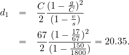
![C [ g]2
δ = -2[1--C]--
1- vs
110[ 29]2
F or phase 1 delay on lane1,δ1 = -2[-1-231100]--= 32.29 sec∕cycle
1- 3000-](web37x.png)
| h | 2.1 | ||||
| s | 1714.3 | ||||
| xc | 0.9 | ||||
| p1 | p1 | p3 | p4 | Cum | |
| L | 2.4 | 2.4 | 2.4 | 2.4 | 9.6 |
| q1 | 300.0 | 120.0 | 180.0 | 170.0 | |
| q2 | 400.0 | 365.0 | 110.0 | 360.0 | |
| q3 | 410.0 | 185.0 | 0.0 | 0.0 | |
| q4 | 110.0 | 450.0 | 0.0 | 0.0 | |
| vci | 410.0 | 450.0 | 180.0 | 360.0 | 1400 |
| v/s | 0.239 | 0.262 | 0.105 | 0.21 | 0.82 |
| Yi | 3.0 | 3.0 | 3.0 | 3.0 | 12.0 |
| C | 103.7 | ||||
| g | 26.8 | 29.5 | 11.8 | 23.6 | 91.7 |
| d | 50.1 | 49.9 | 51.0 | 50.3 | 50.3 |
Solution The through traffic is 50 percent and is equally distributed and left turn has adjustment factor of 1.1 and right turn of 1.4, the calculations are tabulated below:
| Phase | Lane | Flow | Calculation details |
| 1 | 1 | 290.0 | 750x0.5/3 + 750x0.2x1.1 |
| 1 | 2 | 125.0 | 750x0.5/3 |
| 1 | 3 | 440.0 | 750x0.5/3 + 750x0.3x1.4 |
| 2 | 4 | 211.5 | 450x0.5/2 + 450x0.2x1.1 |
| 2 | 5 | 211.5 | 450x0.5/2 + 450x0.3x1.4 |
| 3 | 6 | 232.0 | 600x0.5/3 + 600x0.2x1.1 |
| 3 | 7 | 100.0 | 600x0.5/3 |
| 3 | 8 | 352.0 | 600x0.5/3 + 600x0.3x1.4 |
| 4 | 9 | 141.0 | 300x0.5/2 + 300x0.2x1.1 |
| 4 | 10 | 201.0 | 300x0.5/2 + 300x0.3x1.4 |
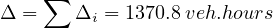
So, the critical flows are 440, 301.5, 352, and 201 respectively for phases 1, 2, 3, and 4. The critical flow for the intersection is sum of all the critical flows for each phase, which is 1294.5 vph.
Solution The saturation flow is 3600/2=1800. The total lost time is 4x4=12. Total green time is 18+13+15+9=55. So the cycle time is 55+12=67.
Effective green time gi=Gi+Y-L=Gi+3-4=Gi-1. So, g1=17, g2=12, g3=14, g4=8.
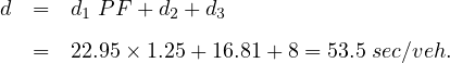
The delay for W-E and S-N approach is shown in the table below. Details of lane 1 is shown below:
| Approach | Lane | Flow | Delay | Cum. Delay |
| W-E | 1 | 150 | 20.35 | 3052.9 |
| W-E | 2 | 350 | 23.16 | 8106.0 |
| W-E | 3 | 250 | 21.67 | 5416.5 |
| Total | 750 | 16575.4 | ||
| S-N | 4 | 200 | 25.40 | 5079.3 |
| S-N | 5 | 280 | 26.73 | 7485.3 |
| Total | 480 | 12564.6 | ||
So, the W-E approach delay is 22.1 seconds per vehicle and S-N approach delay is 26.2 seconds per vehicle.
I wish to thank several of my students and staff of NPTEL for their contribution in this lecture. Specially, I wish to thank my student Mr. Nagraj R for his assistance in developing the lecture note, and my staff Mr. Rayan in typesetting the materials. I also appreciate your constructive feedback which may be sent to tvm@civil.iitb.ac.in
Prof. Tom V. Mathew
Department of Civil Engineering
Indian Institute of Technology Bombay, India
_________________________________________________________________________
Thursday 28 September 2023 10:46:48 AM IST
![[ ( )] ( ) ( )
UD = 1 C 1- g- 2 -vs-- -1--
2 C s- v v C
C-(1---gC)2
= 2 (1- v) (5)
s](web5x.png)