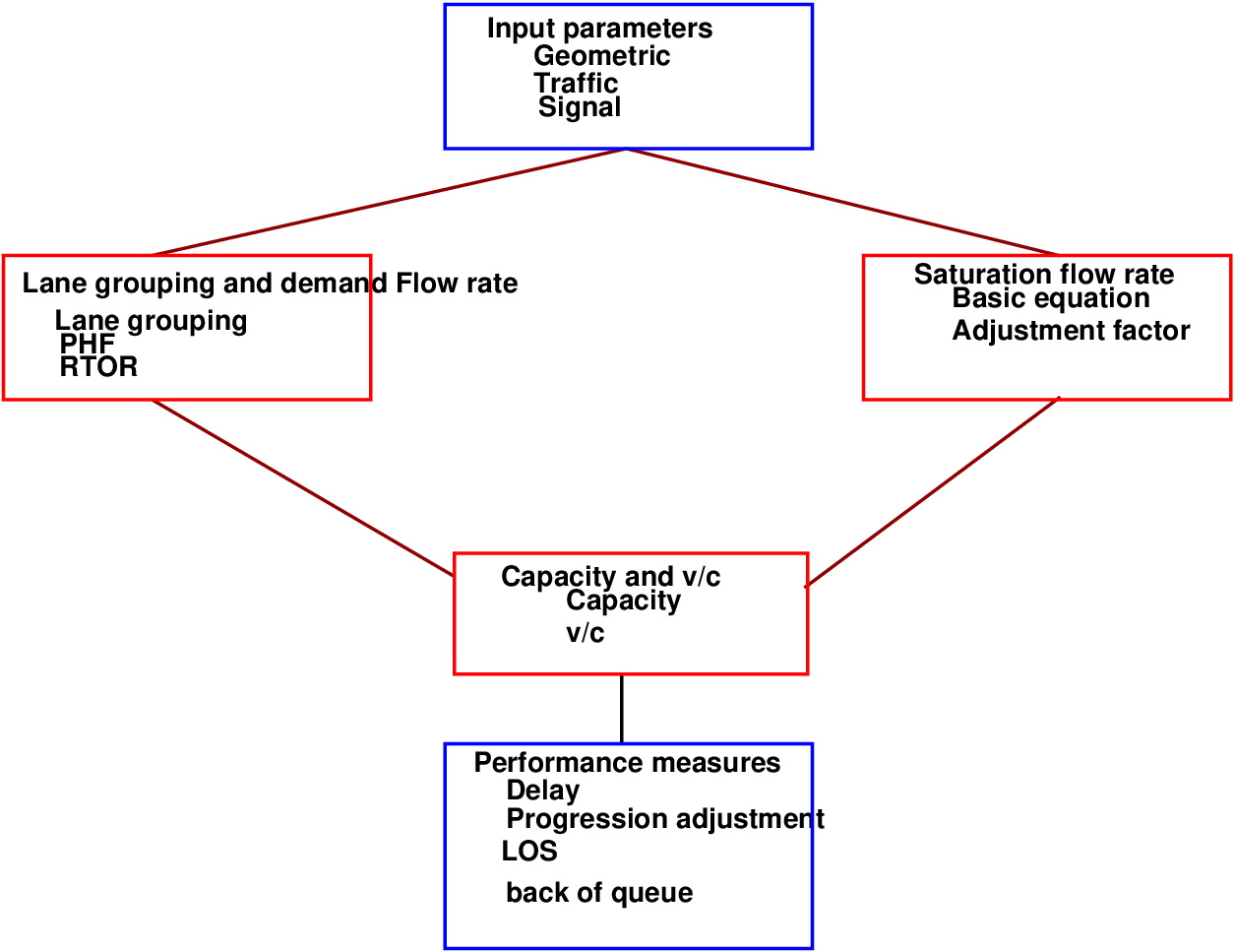
Figure 1: signalized intersection methodology
The Highway Capacity Manual defines the capacity as the maximum howdy rate at which persons or vehicle can be reasonably expected to traverse a point or a uniform segment of a lane or roadway during a given time period, under prevailing roadway, traffic and control conditions. Level-of-Service is introduced by HCM to denote the level of quality one can derive from a local under different operation characteristics and traffic volume.
This chapter contains a methodology for analyzing the capacity and level of service (LOS) of signalized intersections. The analysis must consider a wide variety of prevailing conditions, including the amount and distribution of traffic movements, traffic composition, geometric characteristics, and details of intersection signalization. The methodology focuses on the determination of LOS for known or projected conditions. The capacity analysis methodology for signalized intersections is based on known or projected signalization plans.
The methodology does not take into account the potential impact of downstream congestion on intersection operation. Nor does the methodology detect and adjust for the impacts of turn-pocket overflows on through traffic and intersection operation.
This method uses wide range of operational configuration along with various phase plans, lane utilization, and left-turn treatment alternatives.
The primary output of the method is level of service (LOS). This methodology covers a wide range of operational configurations, including combinations of phase plans, lane utilization, and left-turn treatment alternatives. The below figure shows the signalized intersection methodology.
To conduct operational analysis of signalized intersection, no. of input parameters are required. The data needed are detailed and varied and fall into three main categories: geometric, traffic, and signalization.
| Condition | Parameter |
| Geometric | Area type |
| Number of lanes, N | |
| Average lane width, W (m) | |
| Grade, G (%) | |
| Existence of exclusive LT or RT lanes | |
| Length of storage bay, LT or RT lane, L s (m) | |
| Parking | |
| Traffic | Demand volume by movement, V (veh/h) |
| Base saturation flow rate, s o (pc/h/ln) | |
| Peak-hour factor, PHF | |
| Percent heavy vehicles, HV (%) | |
| Approach pedestrian flow rate, vped (p/h) | |
| Local buses stopping at intersection, NB (buses/h) | |
| Parking activity, Nm (maneuvers/h) | |
| Arrival type, AT | |
| Proportion of vehicles arriving on green, P | |
| Approach speed, S A (km/h) | |
| Control | Cycle length, C (s) |
| Green time, G (s) | |
| Yellow-plus-all-red change-and-clearance interval | |
| (inter green), Y (s) | |
| Actuated or pre-timed operation | |
| Pedestrian push-button | |
| Minimum pedestrian green, Gp (s) | |
| Phase plan | |
| Analysis period, T (h) | |
Intersection geometry is generally presented in diagrammatic form and must include all of the relevant information, including approach grades, the number and width of lanes, and parking conditions.
Traffic volumes (for oversaturated conditions, demand must be used) for the intersection must be specified for each movement on each approach. In situations where the v/c is greater than about 0.9, control delay is significantly affected by the length of the analysis period.
| AT | Description |
| 1 | Dense platoon- 80% arrived at start of red |
| 2 | Moderately dense- 40-80% arrived during red |
| 3 | Less than 40% (highly dispersed platoon) |
| 4 | Moderately dense, 40-80% arrived during green |
| 5 | Dense to moderately dense- 80% arrive at start of green |
| 6 | Very dense platoons progressing over a no. of closed space I/S |
The arrival type should be determined as accurately as possible because it will have a significant impact on delay estimates and LOS determination. It can be computed as
 | (1) |
where, Rp = platoon ratio, P = proportion of all vehicles in movement arriving during green phase, C = cycle length (s) and gi = effective green time for movement or lane group (s).
Complete information regarding signalization is needed to perform an analysis. This information includes a phase diagram illustrating the phase plan, cycle length, green times, and change-and-clearance intervals. If pedestrian timing requirements exist, the minimum green time for the phase is indicated and provided for in the signal timing. The minimum green time for a phase is estimated as,

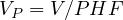
The methodology for signalized intersections is disaggregate; that is, it is designed to consider individual intersection approaches and individual lane groups within approaches. Segmenting the intersection into lane groups is a relatively simple process that considers both the geometry of the intersection and the distribution of traffic movements. Demand volumes are best provided as average flow rates (in vehicles per hour) for the analysis period. However, demand volumes may also be stated for more than one analysis period, such as an hourly volume. In such cases, peaking factors must be provided that convert these to demand flow rates for each particular analysis period. In that case,
 | (3) |
A saturation flow rate for each lane group is computed according to above equation. The saturation flow rate is the flow in vehicles per hour that can be accommodated by the lane group assuming that the green phase were displayed 100 percent of the time (i.e., g/C = 1.0).
 | (4) |
where, s is the saturation flow rate for subject lane group, expressed as a total for all lanes in lane group (veh/h), s0 is the base saturation flow rate per lane (pc/h/ln), N is the number of lanes in lane group, fw is the adjustment factor for lane width, fHV is the adjustment factor for heavy vehicles in traffic stream, fg is the adjustment factor for approach grade, fp is the adjustment factor for existence of a parking lane and parking activity adjacent to lane group, fbb is the adjustment factor for blocking effect of local buses that stop within intersection area, fa is the adjustment factor for area type, fLU is the adjustment factor for lane utilization, fLT is the adjustment factor for left turns in lane group, fRT is the adjustment factor for right turns in lane group, fLpb is the pedestrian adjustment factor for left-turn movements, and fRpb is the pedestrian-bicycle adjustment factor for right-turn movements.
For the analysis of saturation flow rate, a fixed volume is taken as a base called base saturation flow rate, usually 1,900 passenger cars per hour per lane (pc/h/ln). This value is adjusted for a variety of conditions. The adjustment factors are given below.
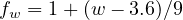
The lane width adjustment factor fw accounts for the negative impact of narrow lanes on saturation flow rate and allows for an increased flow rate on wide lanes. The lane width factor can be calculated for lane width greater than 4.8m. The use of two narrow lanes will always result in higher saturation capacity than one single wide lane.
 | (5) |
where, w = width of lane
passenger cars are affected by approach grades, as are heavy vehicles. The heavy-vehicle factor accounts for the additional space occupied by these vehicles and for the difference in operating capabilities of heavy vehicles compared with passenger cars. The passenger-car equivalent (ET) used for each heavy vehicle is 2.0 passenger-car units and is reflected in the formula. The grade factor accounts for the effect of grades on the operation of all vehicles.
![fHV = 100∕[100+ %HV (ET - 1)] (6)
fg = 1 - %G ∕200 (7)](web5x.png)
Parking maneuver assumed to block traffic for 18 s. Use practical limit of 180 maneuvers/h. The parking adjustment factor, fp, accounts for the frictional effect of a parking lane on flow in an adjacent lane group as well as for the occasional blocking of an adjacent lane by vehicles moving into and out of parking spaces. Each maneuver (either in or out) is assumed to block traffic in the lane next to the parking maneuver for an average of 18 s.
![f = [N - 0.1- (18N ∕3600)]∕N
P m](web6x.png) | (8) |
where, Nm = number of parking maneuvers/h, N = no. of lanes
The bus blockage adjustment factor, fbb, accounts for the impacts of local transit buses that stop to discharge or pick up passengers at a near-side or far-side bus stop within 75 m of the stop line (u/s or d/s). If more than 250 buses per hour exist, a practical limit of 250 should be used. The adjustment factor can be written as,
![fbb = [N - (14.4NB ∕3600)]∕N](web7x.png) | (9) |
where, NB = no. of buses stopping per hour
The area type adjustment factor, fa, accounts for the relative inefficiency of intersections in business districts in comparison with those in other locations. Application of this adjustment factor is typically appropriate in areas that exhibit central business district (CBD) characteristics. It can be represented as, fa = 0.9 in CBD (central business district) and = 1.0 in all others
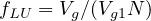
The lane utilization adjustment factor, fLU, accounts for the unequal distribution of traffic among the lanes in a lane group with more than one lane. The factor provides an adjustment to the base saturation flow rate. The adjustment factor is based on the flow in the lane with the highest volume and is calculated by Equation 10.
 | (10) |
where, V g = unadjusted demand flow rate for lane group (veh/ h), V g1 = unadjusted demand flow rate on single lane with highest volume in the lane group and N = no. of lanes in the group.
Capacity at signalized intersections is based on the concept of saturation flow and defined saturation flow rate. The flow ratio for a given lane group is defined as the ratio of the actual or projected demand flow rate for the lane group (vi) and the saturation flow rate(si). The flow ratio is given the symbol (v/s)i for lane group i. Capacity at signalized I/S is based on the saturation flow and saturation flow rate.
 | (11) |
where ci = capacity of lane group i (veh/h), si = saturation flow rate for lane group i (veh/h) and gi∕C = effective green ratio for lane group i.
The ratio of flow rate to capacity (v/c), often called the volume to capacity ratio, is given the symbol X in intersection analysis
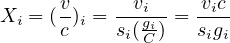 | (12) |
where, Xi = (v/c)i = ratio for lane group i, vi = actual or projected demand flow rate for lane group i (veh/h), si = saturation flow rate for lane group i (veh/h), gi = effective green time for lane group i (s) and C = cycle length (s)
Another concept used for analyzing signalized intersections is the critical v/c ratio, Xc. This is the v/c ratio for the intersection as a whole, considering only the lane groups that have the highest flow ratio (v/s) for a given signal phase. For example, with a two-phase signal, opposing lane groups move during the same green time. Generally, one of these two lane groups will require more green time than the other (i.e., it will have a higher flow ratio). This would be the critical lane group for that signal phase. The critical v/c ratio for the intersection is determined by using Equation,
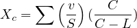 | (13) |
where, Xc = critical v/c ratio for intersection; The above eqn. is useful in evaluating the overall i/s w.r.t the geometric and total cycle length. A critical v/c ratio less than 1.0, however, does indicate that all movements in the intersection can be accommodated within the defined cycle length.
The values derived from the delay calculations represent the average control delay experienced by all vehicles that arrive in the analysis period, including delays incurred beyond the analysis period when the lane group is oversaturated. The average control delay per vehicle for a given lane group is given by Equation,
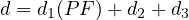 |
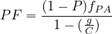
where, d = control delay per vehicle (s/veh); d1 = uniform control delay assuming uniform arrivals (s/veh); PF = uniform delay progression adjustment factor, d2 = incremental delay to account for effect of random arrivals and d3 = initial queue delay, which accounts for delay to all vehicles in analysis period
Good signal progression will result in a high proportion of vehicles arriving on the uniform delay Green and vice-versa. Progression primarily affects uniform delay, and for this reason, the adjustment is applied only to d1. The value of PF may be determined using Equation,
 | (14) |
where, PF = progression adjustment factor, P = proportion of vehicles arriving on green, g/C = proportion of green time available, fPA = supplemental adjustment factor for platoon arriving during green. The approximate ranges of RP are related to arrival type as shown below.
| AT | Ration | Default Rp | Progression quality |
| 1 | ≤ 0.50 | 0.333 | very poor |
| 2 | 0.50-0.85 | 0.667 | Unfavorable |
| 3 | 0.85-1.15 | 1.000 | Random arrivals |
| 4 | 1.15-1.50 | 1.333 | Favorable |
| 5 | 1.50-2.00 | 1.667 | Highly favorable |
| 6 | 2.00 | 2.000 | Exceptional |
PF may be calculated from measured values of P using the given values of fPA or the following table can be used to determine PF as a function of the arrival type.
| Green Ratio | ||||||
| (g/C) | AT1 | AT2 | AT3 | AT4 | AT5 | AT6 |
| 0.2 | 1.167 | 1.007 | 1 | 1 | 0.833 | 0.75 |
| 0.3 | 1.286 | 1.063 | 1 | 0.986 | 0.714 | 0.571 |
| 0.4 | 1.445 | 1.136 | 1 | 0.895 | 0.555 | 0.333 |
| 0.5 | 1.667 | 1.24 | 1 | 0.767 | 0.333 | 0 |
| 0.6 | 2.001 | 1.395 | 1 | 0.576 | 0 | 0 |
| 0.7 | 2.556 | 1.653 | 1 | 0.256 | 0 | 0 |
| fPA | 1 | 0.93 | 1 | 1.15 | 1 | 1 |
| Default, Rp | 0.333 | 0.667 | 1 | 1.333 | 1.667 | 2 |
It is based on assuming uniform arrival, uniform flow rate & no initial queue. The formula for uniform delay is,
![g-2
d1 = --0.5C-(1---C)-g-
1- [min(1,X )C]](web14x.png) | (15) |
where, d1 = uniform control delay assuming uniform arrivals (s/veh), C = cycle length (s); cycle length used in pre-timed signal control, g = effective green time for lane group, X = v/c ratio or degree of saturation for lane group.
The equation below is used to estimate the incremental delay due to nonuniform arrivals and temporary cycle failures (random delay. The equation assumes that there is no unmet demand that causes initial queues at the start of the analysis period (T).
![[ ∘ --------------]
2 8klX--
d2 = 900 T (X - 1)+ (X - 1) + cT](web15x.png) | (16) |
where, d2 = incremental delay queues, T = duration of analysis period (h); k = incremental delay factor that is dependent on controller settings, I = upstream filtering/metering adjustment factor; c = lane group capacity (veh/h), X = lane group v/c ratio or degree of saturation, and K can be found out from the following table.
| Unit | ||||||
| Extension (s) | ≤ 0.50 | 0.6 | 0.7 | 0.8 | 0.9 | ≥ 1.0 |
| ≤ 2.0 | 0.04 | 0.13 | 0.22 | 0.32 | 0.41 | 0.5 |
| 2.5 | 0.08 | 0.16 | 0.25 | 0.33 | 0.42 | 0.5 |
| 3 | 0.11 | 0.19 | 0.27 | 0.34 | 0.42 | 0.5 |
| 3.5 | 0.13 | 0.2 | 0.28 | 0.35 | 0.43 | 0.5 |
| 4 | 0.15 | 0.22 | 0.29 | 0.36 | 0.43 | 0.5 |
| 4.5 | 0.19 | 0.25 | 0.31 | 0.38 | 0.44 | 0.5 |
| 5.0a | 0.23 | 0.28 | 0.34 | 0.39 | 0.45 | 0.5 |
| Pre-timed | 0.5 | 0.5 | 0.5 | 0.5 | 0.5 | 0.5 |
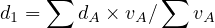
The delay obtained has to be aggregated, first for each approach and then for the intersection The weighted average of control delay is given as:
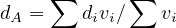 |
where, di = delay per vehicle for each movement (s/veh), dA = delay for Approach A (s/veh), and vA = adjusted flow for Approach A (veh/h).
 |
Intersection LOS is directly related to the average control delay per vehicle. Any v/c ratio greater than 1.0 is an indication of actual or potential breakdown. In such cases, multi-period analyses are advised. These analyses encompass all periods in which queue carryover due to oversaturation occurs. A critical v/c ratio greater than 1.0 indicates that the overall signal and geometric design provides inadequate capacity for the given flows. In some cases, delay will be high even when v/c ratios are low.
| LOS | Delay |
| A | ≤ 10 |
| B | 10-20 |
| C | 20-35 |
| D | 35-55 |
| E | 55-80 |
| F | >80 |
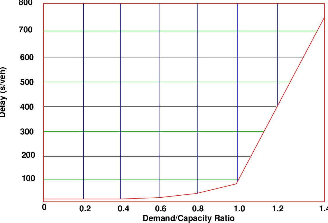
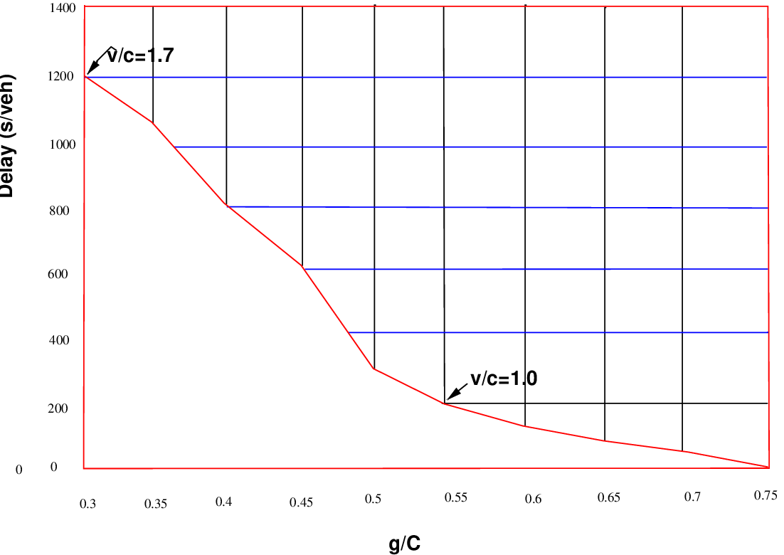
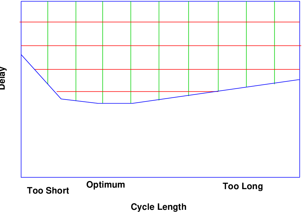
The predicted delay is highly sensitive to signal control characteristics and the quality of progression. The predicted delay is sensitive to the estimated saturation flow only when demand approaches or exceeds 90 percent of the capacity for a lane group or an intersection approach. The following graph shows the sensitivity of the predicted control delay per vehicle to demand to capacity ratio, g/c, cycle length and length of analysis period.
Assumptions are : Cycle length = 100s, g/c = 0.5, T =1h, k = 0.5, l= 1, s = 1800 veh/hr
HCM model is very useful for the analysis of signalized intersection as it considers all the adjustment factors which are to be taken into account while designing for a signalized I/S. Though,the procedure is lengthy but it is simple in approach and easy to follow.
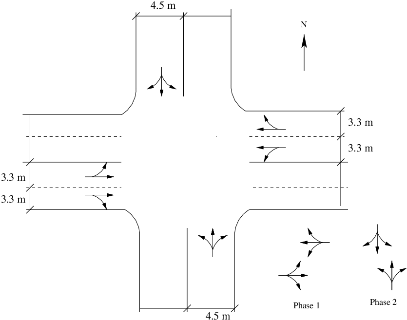
The intersection is located in CBD area and the traffic volume in each direction in vehicles/hour is given as
| East | West | North | South | |
| bound | bound | bound | bound | |
| Left turn | 65 | 30 | 30 | 40 |
| Through | 620 | 700 | 370 | 510 |
| Right turn | 35 | 20 | 20 | 50 |
Pedestrian volume = 100 pedestrains/hour,
Percentage of heavy vehicles = 5% in East and West approaches and 8% in North and
South approaches,
Base saturation flow rate = 1900 veh/h/lane,
Peak hour factor= 0.9,
Cross walk width = 3.0 m,
North bound and South bound has two lanes, one in each direction of lane width
4.5m,
East bound and West bound has four lanes, two in each direction of lane width
3.3m.
Two phase signal with cycle time 70 seconds and North bound-South bound green
time=36 s,
East bound-West bound green time =26 s,
Amber time= 4 s and Movement lost time =4 s,
Arrival type 4 and Analysis duration = 15 min,
Assume 0% grade with no parking maneuvers and no buses stopping.
Consider Lane utilisation adjustment factor in North and South approaches= 1.00, East
and West approaches = 0.95.
Left turn pedestrian/bicycle adjustment factor= 0.999(N), 0.998(S), 0.997(E),
0.998(W),
Right turn pedestrian/bicycle adjustment factor= 0.996(N), 0.994(S), 0.992(E),
0.995(W),
Passenger car equivalent for heavy vehicle = 2.0,
Left turn adjustment factor is 0.937(N), 0.951(S), 0.716(E), 0.901(W).
Incremental delay factor= 0.5 and Initial queue delay= 0 s/veh.
Progression adjustment factor = 1.000.
I wish to thank several of my students and staff of NPTEL for their contribution in this lecture. I also appreciate your constructive feedback which may be sent to tvm@civil.iitb.ac.in
Prof. Tom V. Mathew
Department of Civil Engineering
Indian Institute of Technology Bombay, India
_________________________________________________________________________
Thursday 28 September 2023 10:47:21 AM IST