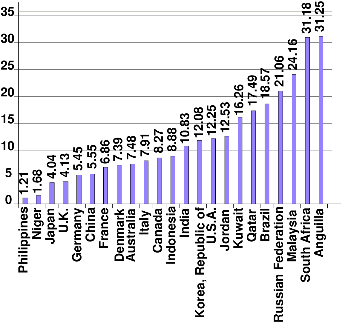
Figure 1: Country-wise number of person killed per 100000 populations (Ref. Ministry
of Road Transport and Highways Transport Research Wing)
This lecture covers one of the most important negative impact of transportation system, namely the accidents. This lecture first presents some introductory stuff including some salient accident statistics, causes of accidents, accident data collection, accident reconstruction, safety measures and safety audit.
The problem of accident is a very acute in highway transportation due to complex flow pattern of vehicular traffic, presence of mixed traffic along with pedestrians. Traffic accident leads to loss of life and property. Thus the traffic engineers have to undertake a big responsibility of providing safe traffic movements to the road users and ensure their safety. Road accidents cannot be totally prevented but by suitable traffic engineering and management the accident rate can be reduced to a certain extent. For this reason systematic study of traffic accidents are required to be carried out. Proper investigation of the cause of accident will help to propose preventive measures in terms of design and control.
Some objectives of accident studies are listed below:
The various causes of road accidents are:
The statistical analysis of accident is carried out periodically at critical locations or road stretches which will help to arrive at suitable measures to effectively decrease accident rates. It is the measure (or estimates) of the number and severity of accident. These statistics reports are to be maintained zone-wise. Accident prone stretches of different roads may be assessed by finding the accident density per length of the road. The places of accidents are marked on the map and the points of their clustering (BLACK SPOT) are determined. By statistical study of accident occurrence at a particular road or location or zone of study for a long period of time it is possible to predict with reasonable accuracy the probability of accident occurrence per day or relative safety of different classes of road user in that location. The interpretation of the statistical data is very important to provide insight to the problem. The position of India in the year 2009 in country-wise number of person killed per 100000 populations as shown in the Figure 1 and the increase in rate of accident from year 2005 to year 2009 is shown in the table. 1. In 2009, 14 accidents occurred per hour.
| No. of Accidents | No. of persons affected | Accident severity | |||
| Year | Total | Fatal | Killed | Injured | (No. of persons killed |
| per 100 accidents) | |||||
| 2005 | 4,39,255 | 83,491 | 94,968 | 4,65,282 | 22 |
| 2006 | 4,60,920 | 93,917 | 1,05,749 | 4,96,481 | 23 |
| 2007 | 4,79,216 | 1,01,161 | 1,14,444 | 5,13,340 | 24 |
| 2008 | 4,84,704 | 1,06,591 | 1,19,860 | 5,23,193 | 25 |
| 2009 | 4,86,384 | 1,10,993 | 1,25,660 | 5,15,458 | 25.8 |
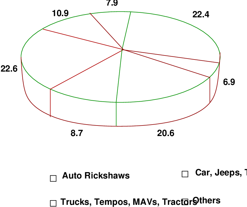
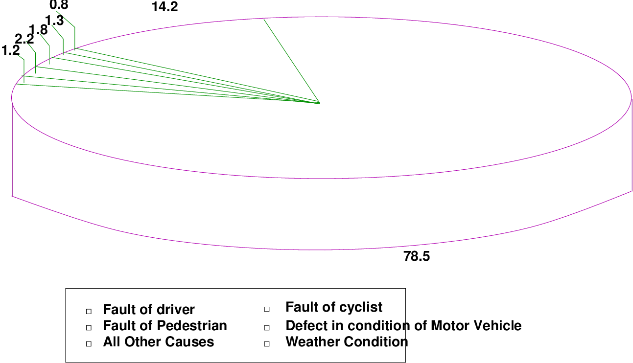
Figure 2 and 3 gives the percent of accident occurring from a specific vehicle class and the causes of accident in the form of pie-chart. Since the data collection of accident is mostly done by the traffic police it’s the users who are put to blame in majority of cases. Thus such statistical records are not much useful for the traffic engineer.
The accident data collection is the first step in the accident study. The data collection of the accidents is primarily done by the police. Motorist accident reports are secondary data which are filed by motorists themselves. The data to be collected should comprise all of these parameters:
These data collected need proper storing and retrieving for the following purpose. The purposes are as follows:
The accident data collection involves extensive investigation which involves the following procedure:
The purpose is to find the possible causes of accident related to driver, vehicle, and roadway. Accident analyses are made to develop information such as:
It is important to compute accident rate which reflect accident involvement by type of highway. These rates provide a means of comparing the relative safety of different highway and street system and traffic controls. Another is accident involvement by the type of drivers and vehicles associated with accidents.
 | (1) |
where, R = total accident rate per km for one year, A = total number of accident
occurring in one year, L = length of control section in kms
 | (2) |
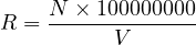
where,R = accident involvement per 100 million vehicle-kms of travel, N = total number
of drivers of vehicles involved in accidents during the period of investigation and
V = vehicle-kms of travel on road section during the period of investigation
 | (3) |
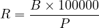
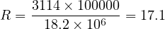
where, R = death rate per 100,000 population, B = total number of traffic death in one
year and P = population of area
 | (4) |
where, R = death rate per 10,000 vehicles registered, B = total number of traffic
death in one year and M = number of motor vehicles registered in the area
 | (5) |
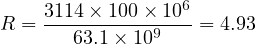
where, R = accident rate per 100 million vehicle kms of travel, C = number of total
accidents in one year and V = vehicle kms of travel in one year
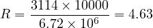
The Motor vehicle consumption in a city is 5.082 million liters, there were 3114 motor vehicle fatalities, 355,799 motor vehicle injuries, 6,721,049 motor vehicle registrations and an estimated population of 18,190,238. Kilometer of travel per liter of fuel is 12.42 km/liter. Calculate registration death rate, population death rate and accident rate per vehicle km.
Solution Approximate vehicle kms of travel = Total consumption o fuel × kilometer of travel per liter of fuel =5.08 × 109 × 12.42 = 63.1 × 10⁹ km.
Accident reconstruction deals with representing the accidents occurred in schematic diagram to determine the pre-collision speed which helps in regulating or enforcing rules to control or check movement of vehicles on road at high speed. The following data are required to determine the pre-collision speed:
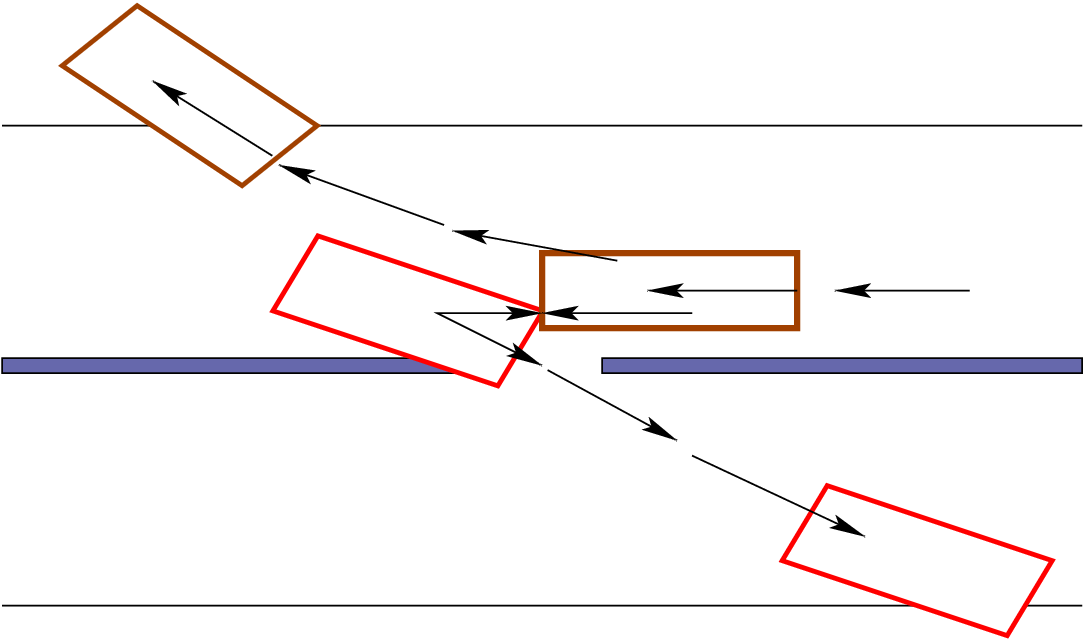
Below in Figure 4 a schematic diagram of collision of two vehicles is shown that occur during turning movements. This diagram is also known as collision diagram. Each collision is represented by a set of arrows to show the direction of before and after movement. The collision diagram provides a powerful visual record of accident occurrence over a significant period of time.
The collision may be of two types collinear impact or angular collision. Below each of them are described in detail. Collinear impact can be again divided into two types :
It can be determined by two theories:
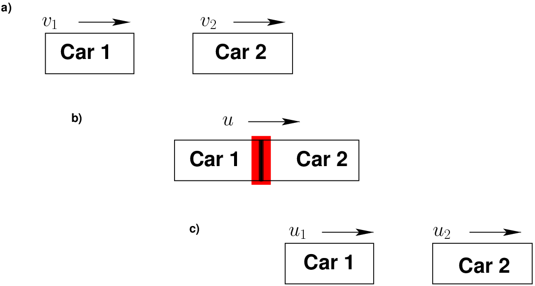
Poisson impact theory, divides the impact in two parts - compression and restitution. The Figure 5 shows two vehicles travelling at an initial speed of v1 and v2 collide and obtain a uniform speed say u at the compression stage. And after the compression stage is over the final speed is u1 and u2. The compression phase is cited by the deformation of the cars.
From the Newton’s law F = ma,
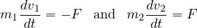 | (6) |
where, m1 and m2 are the masses of the cars and F is the contact force. We know that every reaction has equal and opposite action. So as the rear vehicle pushes the vehicle ahead with force F. The vehicle ahead will also push the rear vehicle with same magnitude of force but has different direction. The action force is represented by F, whereas the reaction force is represented by -F as shown in Figure 6.
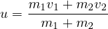
In the compression phase cars are deformed. The compression phase terminates when the cars have equal velocity. Thus the cars obtain equal velocity which generates the following equation:
 | (7) |
where, Pc ≡∫ 0τcF dt which is the compression impulse and τc is the compression time. Thus, the velocity after collision is obtained as:
 | (8) |
The compression impulse is given by:
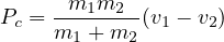 | (9) |
In the restitution phase the elastic part of internal energy is released
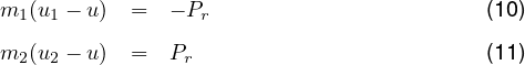
where, Pr ≡∫ 0τrF dt is the restitution impulse and τr is the restitution time. According to Poisson’s hypothesis restitution impulse is proportional to compression impulse
 | (12) |
Restitution impulse e is given by:
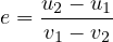 | (13) |
The total impulse is P = Pc + Pr
 | (14) |
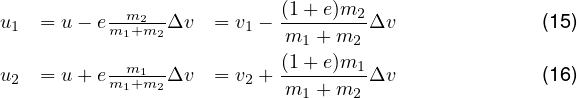
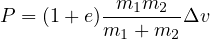
The post impact velocities are given by:
where Δv = v1 - v2. But we are required to determine the pre-collision speed according to which the safety on the road can be designed. So we will determine v1 and v2 from the given value of u1 and u2 .Two vehicles travelling in the same lane have masses 3000 kg and 2500 kg. The velocity of rear vehicles after striking the leader vehicle is 25 kmph and the velocity of leader vehicle is 56 kmph. The coefficient of restitution of the two vehicle system is assumed to be 0.6. Determine the pre-collision speed of the two vehicles.
Solution Given that the: mass of the first vehicle (m1) = 3000 kg, mass of the second vehicle (m2) = 2500 kg, final speed of the rear vehicle (u1) = 25 kmph, and final speed of the leader vehicle (u2) = 56 kmph. Let initial speed of the rear vehicle be v1, and let initial speed of the leader vehicle be v2.
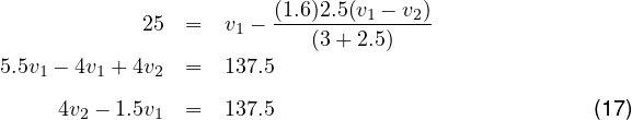
Step 1: From equation. 15,
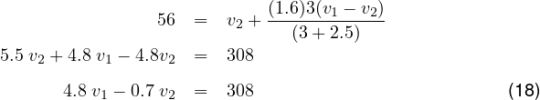
Step 2: From equation. 16,
Step 3: Solving equations. 17 and 18, We get the pre collision speed of two vehicles as: v1 = 73 kmph, and v2 = 62 kmph.
Step 4: Initial speed of the rear vehicle, v1 = 73 kmph, and the initial speed of leader vehicle, v2 = 62 kmph. Thus from the result we can infer that the follower vehicle was travelling at quite high speed which may have resulted in the collision. The solution to the problem may be speed restriction in that particular stretch of road where accident occurred.
Applying principle of conservation of energy or conservation of momentum also the initial speed of the vehicle can be computed if the skid marks are known. It is based on the concept that there is reduction in kinetic energy with the work done against the skid resistance. So if the vehicle of weight W slow down from speed v1 to v2, then the loss in kinetic energy will be equal to the work done against skid resistance, where work done is weight of the vehicle multiplied by the skid distance and the skid resistance coefficient.
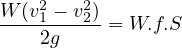 | (19) |
where, f is the skid resistance coefficient and S is the skid distance. It also follows the law of conservation of momentum (m1, v1 are the mass and velocity of first vehicle colliding with another vehicle of mass and velocity m2, v2 respectively)
 | (20) |
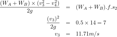
A vehicle of 2000 kg skids a distance of 36 m before colliding with a stationary vehicle of 1500
kg weight. After collision both vehicle skid a distance of 14 m. Assuming coefficient of friction
0.5, determine the initial speed of the vehicle.
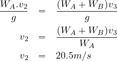
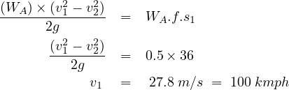
Solution: Let the weight of the moving vehicle is WA, let the weight of the stationary vehicle is WB, skid distance before and after collision is s1 and s2 respectively, initial speed is v1, speed after applying brakes before collision is v2 and the speed of both the vehicles A and B after collision is v3, and the final speed v4 is 0. Then:
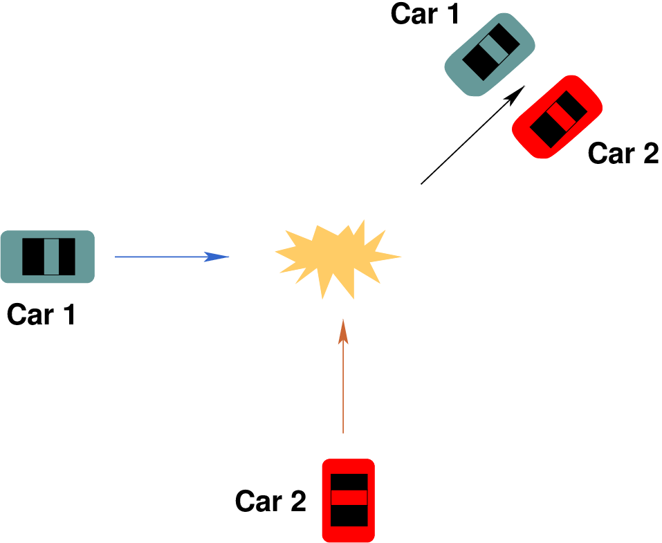
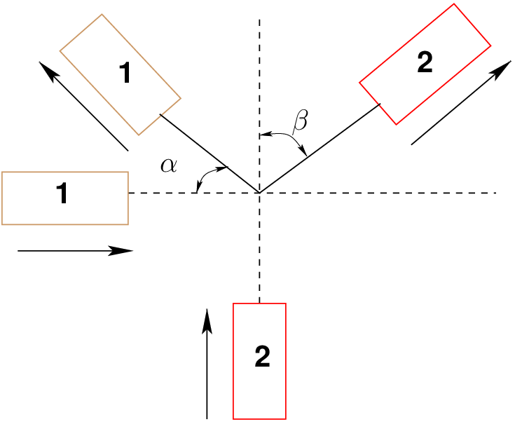
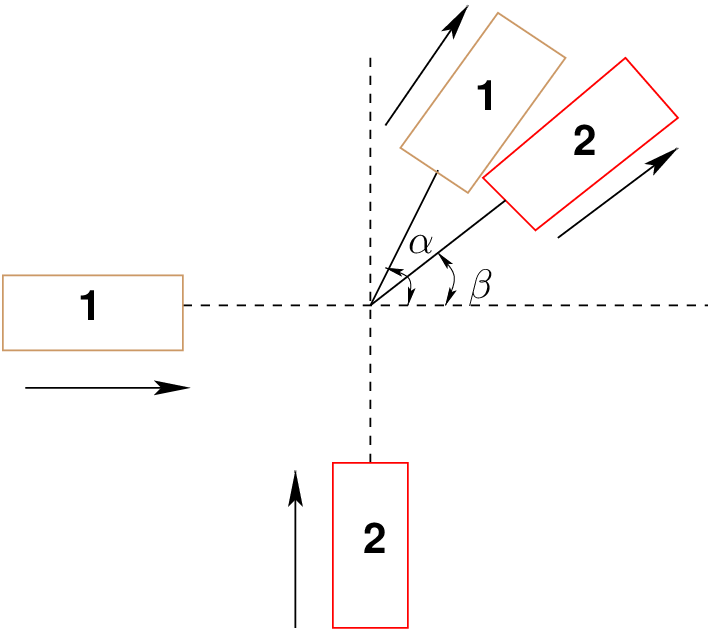
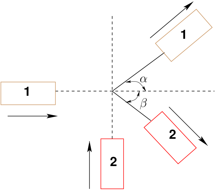
Angular collision occurs when two vehicles coming at right angles collies with each other and
bifurcates in different direction. The direction of the vehicles after collision in this case
depends on the initial speeds of the two vehicles and their weights. One general case is that
two vehicles coming from south and west direction after colliding move in its resultant
direction as shown in Figure 7.
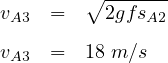
The mass of the car 1 is m1 kg and the car 2 is m2 kg and the initial velocity is v1 m/s and
v2 m/s respectively. So as the momentum is the product of mass and velocity. The momentum
of the car 1 and car 2 is m1v1 kgm/s and m2v2 kgm/s respectively. By the law of conservation
of momentum the final momentum should be equal to the initial momentum. But as the car are
approaching each other at an angle the final momentum should not be just mere
summation of both the momentum but the resultant of the two, Resultant momentum =
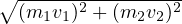 kg m/s. The angle at which they are bifurcated after collision
is given by tan-1(h∕b) where h is the hypotenuse and b is the base. Therefore,
the cars are inclined at an angle. Inclined at an angle = tan-1(m2v2∕m1v1). Now,
since the mass of the two vehicles are same the final velocity will proportionally be
changed. The general schematic diagrams of collision are shown in Figs. 8 to 10.
kg m/s. The angle at which they are bifurcated after collision
is given by tan-1(h∕b) where h is the hypotenuse and b is the base. Therefore,
the cars are inclined at an angle. Inclined at an angle = tan-1(m2v2∕m1v1). Now,
since the mass of the two vehicles are same the final velocity will proportionally be
changed. The general schematic diagrams of collision are shown in Figs. 8 to 10.
Vehicle A is approaching from west and vehicle B from south. After collision A skids 600 north of east and B skids 300 south of east as shown in Figure 10. Skid distance before collision for A is 18 m and B is 26 m. The skid distances after collision are 30m and 15 m respectively. Weight of A and B are 4500 and 6000 respectively. Skid resistance of pavement is 0.55 m. Determine the pre-collision speed.
Solution Let: initial speed is vA1 and vB1, speed after skidding before collision is vA2 and vB2, speed of both the vehicles A and B after collision is vA3 and vB3, final speed is vA4 and vB4 is 0, initial skid distance for A and B is sA1 and sB1, final skid distance for A and B is sA2 and sB2, and weight of vehicle A is WA and Weight of vehicle B is WB.
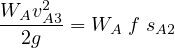
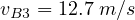
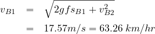
Answer: The pre-collision speed of the vehicle A (approaching from west) is vA1 = 99 km/hr and vehicle B (approaching from south) is vB1 = 63.26 km/hr.
The ultimate goal is to develop certain improvement measures to mitigate the circumstances leading to the accidents. The measures to decrease the accident rates are generally divided into three groups engineering, enforcement and education. Some safety measures are described below:
The various measures of engineering that may be useful to prevent accidents are enumerated below
There is consecutive change of picture in driver’s mind while he is in motion. The number of factors that the driver can distinguish and clearly fix in his mind is limited. On an average the perception time for vision is 1∕16th, for hearing is 1∕20th and for muscular reaction is 1∕20th. The number of factors that can be taken into account by organs of sense of a driver in one second is given by the formula below.
 | (21) |
where, M = No. of factors that can be taken into account by the organ of sense of driver for L m long, V = speed of vehicle in m/sec. Factors affecting drivers’ attention when he is on road can be divided into three groups:
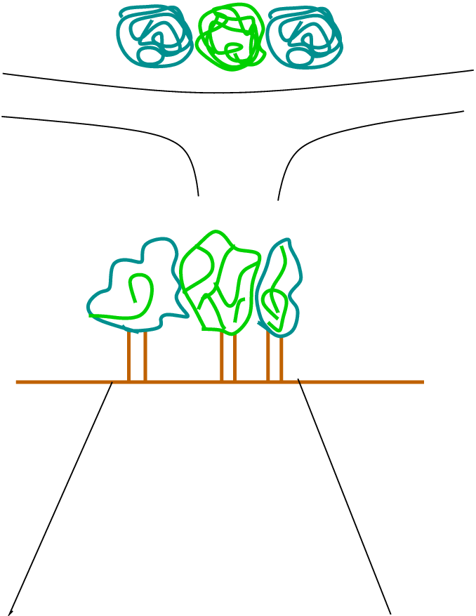
So using the laws of visual perception certain measures have been suggested:
Figure 11 and 12 is a visual guidance measure. Planting trees along side of roadway which has a turning angle attracts attention of the driver and signals that a turn is present ahead.
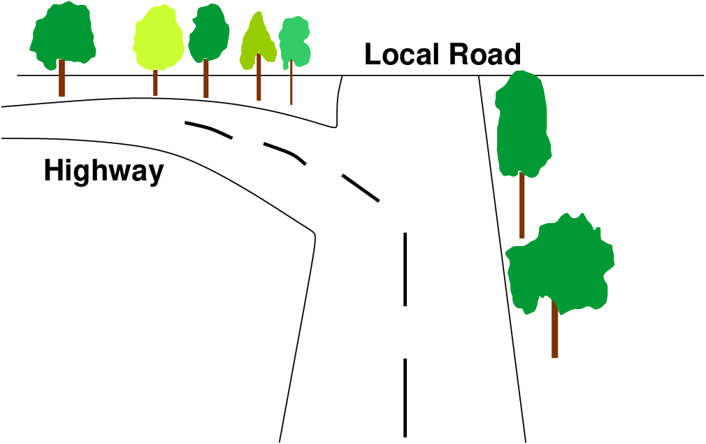
The figure below is another example, when the direction of road has a hazardous at-grade intersection trees are planted in such a way that it seems that there is dense forest ahead and driver automatically tends to stop or reduce the speed of the vehicle so that no conflicts occur at that point.
Driver tends to extrapolate the further direction of the road. So it is the responsibility of the traffic engineer to make the driver psychologically confident while driving that reduces the probability of error and prevent mental strain.
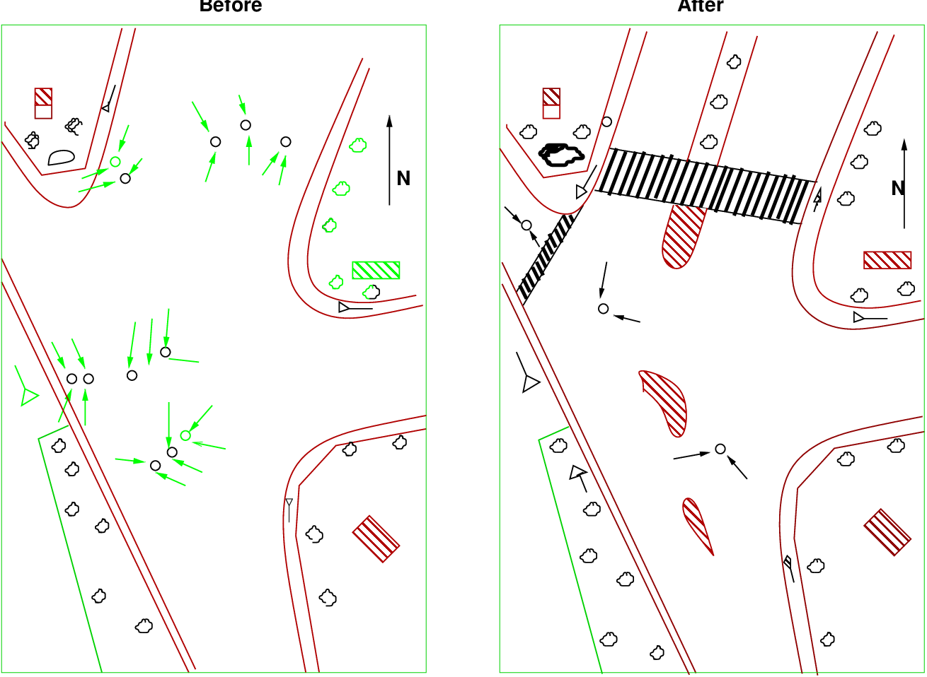
The number of vehicles on the road increases from year to year, which introduces complications into organization of traffic, sharply reduces the operation and transportation characteristic of roads and lead to the growth of accident rate. This leads to the need of re constructing road. The places of accidents need to be properly marked so that the reconstruction can be planned accordingly.
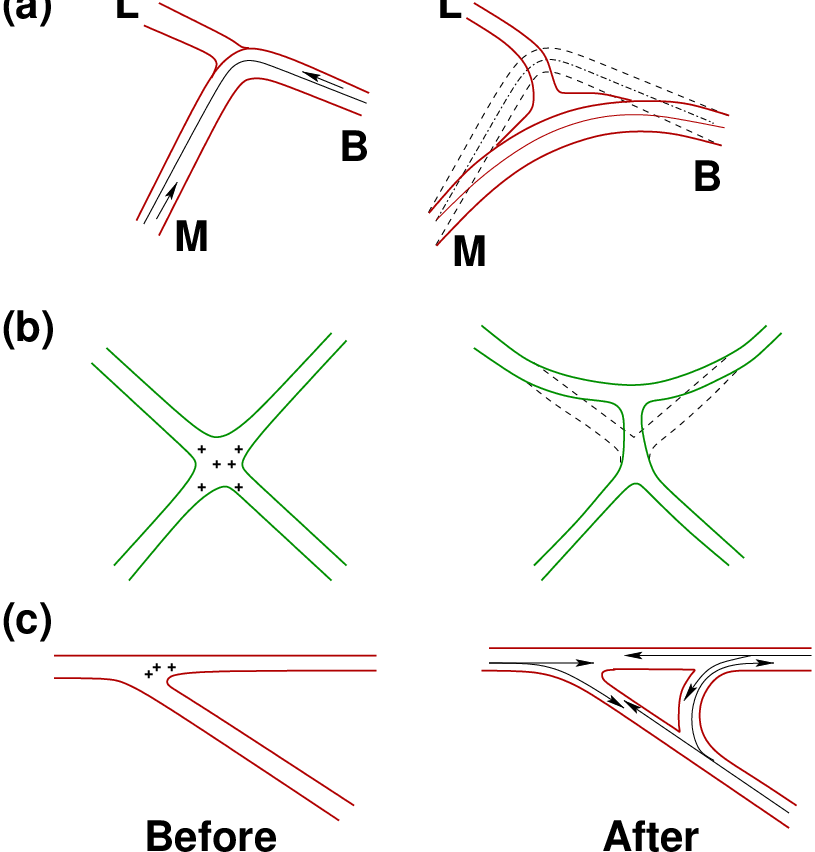
The Figure 13 shows that there were too many conflict points before which reduced to a few number after construction of islands at proper places. Reconstruction process may also include construction of a new road next to the existing road, renewal of pavement without changing the horizontal alignment or profile of the road, reconstruction a particular section of road. Few more examples of reconstruction of selected road section to improve traffic safety are shown in Figure 14.
The Figure 14 (a) shows separation of direction of main stream of traffic from the secondary ones by shifting place of three-leg intersection, Figure 14(b) shows separation of roads with construction of connection between them and Figure 14(c) shows the construction of additional lane for turning vehicles. The plus sign indicates the conflict points before the road reconstruction has been carried out. The after reconstruction figure shows that just by little alteration of a section of road how the conflict points have been resolved and smooth flow of the vehicles in an organized manner have been obtained.
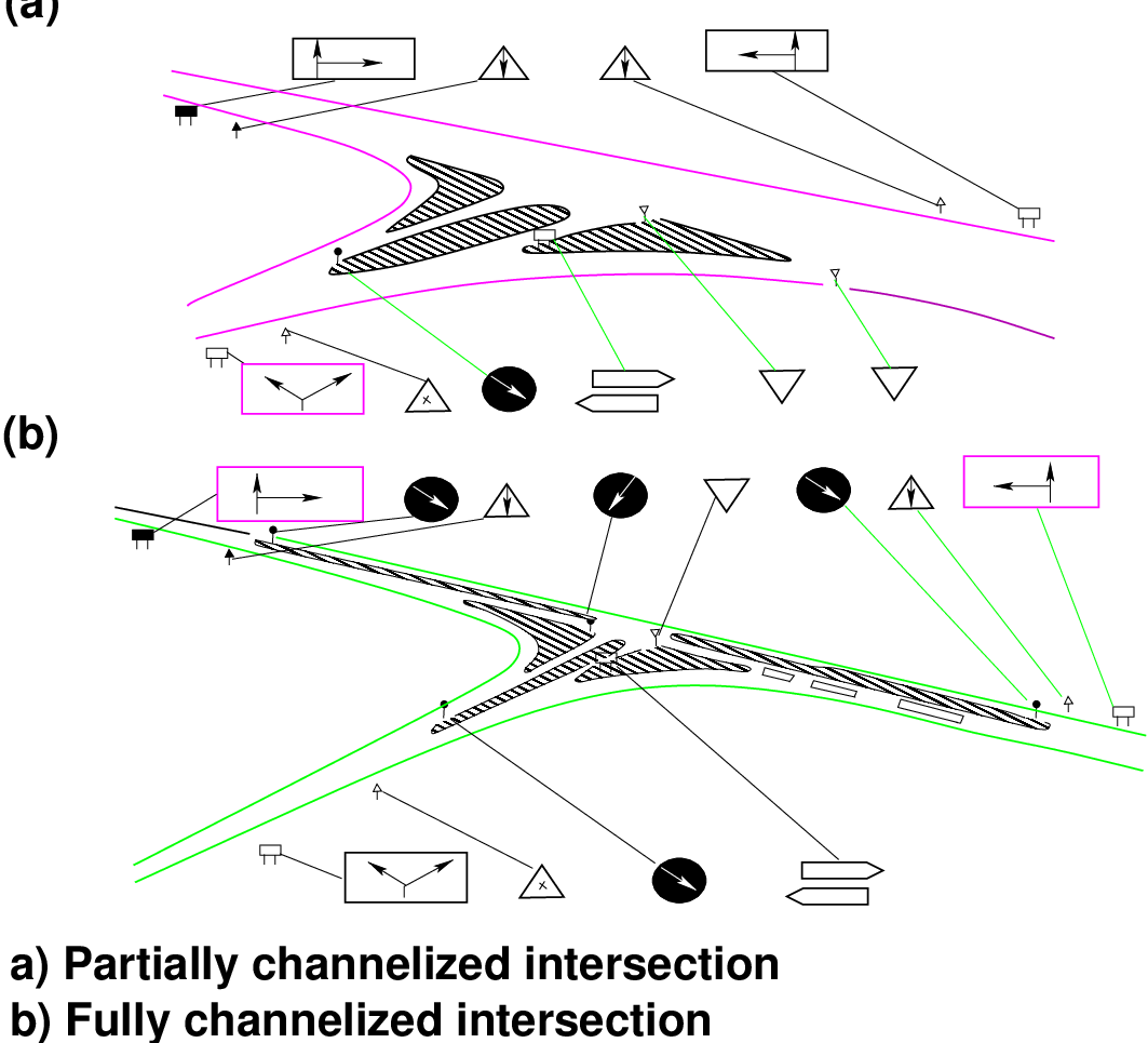
The Channelization of traffic at intersection separates the traffic stream travelling in different direction, providing them a separate lane that corresponds to their convenient path and spreading as far as possible the points of conflict between crossing traffic streams. The traffic lanes are separated by marking relevant lines or by constructing slightly elevated islands as shown in Figure 15. Proper Channelization reduces confusion. The number of decision required to be made by the driver at any time is reduced allowing the driver time to make next decision. The principles of proper channelized intersection are:-
Road signs are integral part of safety as they ensure safety of the driver himself (warning signs) and safety of the other vehicles and pedestrians on road (regulatory signs). Driver should be able to read the sign from a distance so that he has enough time to understand and respond. It is essential that they are installed and have correct shape, colour, size and location. It is required to maintain them as well, without maintenance in sound condition just their installment would not be beneficial. According to British investigation height of text in road sign should be
Various other methods of traffic accident mitigation are described below:
The various measures of enforcement that may be useful to prevent accidents at spots prone to accidents are enumerated below. These rules are revised from time to time to make them more comprehensive.
Checks on spot speed of all vehicles should be done at different locations and timings and legal actions on those who violate the speed limit should be taken
The transport authorities should be strict while issuing licence to drivers of public service vehicles and taxis. Driving licence of the driver may be renewed after specified period, only after conducting some tests to check whether the driver is fit
The drivers should be tested for vision and reaction time at prescribed intervals of time
The various measures of education that may be useful to prevent accidents are enumerated below.
The passengers and pedestrians should be taught the rules of the road, correct manner of crossing etc. by introducing necessary instruction in the schools for the children and by the help of posters exhibiting the serious results due to carelessness of road users.
Imposing traffic safety week when the road users are properly directed by the help of traffic police as a means of training the public. Training courses and workshops should be organized for drivers in different parts of the country.
It is the procedure of assessment of the safety measures employed for the road. It has the advantages like proper planning and decision from beforehand ensures minimization of future accidents, the long term cost associated with planning is also reduced and enables all kinds of users to perceive clearly how to use it safely. Safety audit takes place in five stages as suggested by Wrisberg and Nilsson, 1996. Five Stages of Safety Audit are:
An example of safety audit is discussed below.
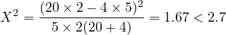
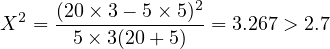
To estimate the effectiveness of improvement of dangerous section the number of accidents before and after is compared. To do this Chi Square test is used to check whether the experimental data meet the allowable deviation from the theoretical analysis. In the simplest case one group of data before and after road reconstruction is considered.
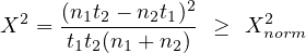 | (22) |
where, t1 and t2 = period of time before and after reconstruction of a stretch of road for which statistical data of accident is available, n1 and n2 = corresponding numbers of accident, Xnorm2 = minimum values of Chi Square at which probability of deviation of laws of accident occurrence after reconstruction P from the laws existing before reconstruction does not exceed permissible values (usually 5%) The relationship between P and Xnorm2 is shown in Table. 2.
| P | 10 | 8 | 5 | 3 | 2 | 1 | 0.1 |
| Xnorm2 | 1.71 | 2 | 2.7 | 3.6 | 4.25 | 5.41 | 9.6 |
Before reconstruction of an at-grade intersection, there were 20 accidents during 5 years. After reconstruction there were 4 accidents during 2 years. Determine the effectiveness of the reconstruction.
Solution: Using Chi square test, we have (with P = 5 %)
This chapter provides an important subject of highway safety and accident studies. Everything a traffic engineer does, from field studies, planning and design; to control operation is related to the provision of the safety system for vehicular travel. This chapter gives an insight of how the analysis of traffic accident can be done from the viewpoint to reduce it by designing proper safety measure.
I wish to thank several of my students and staff of NPTEL for their contribution in this lecture. Specially, I wish to thank my student Ms. Apurba Ghosh for his assistance in developing the lecture note, and my staff Ms. Reeba in typesetting the materials. I also appreciate your constructive feedback which may be sent to tvm@civil.iitb.ac.in
Prof. Tom V. Mathew
Department of Civil Engineering
Indian Institute of Technology Bombay, India
_________________________________________________________________________
Thursday 28 September 2023 11:39:23 AM IST