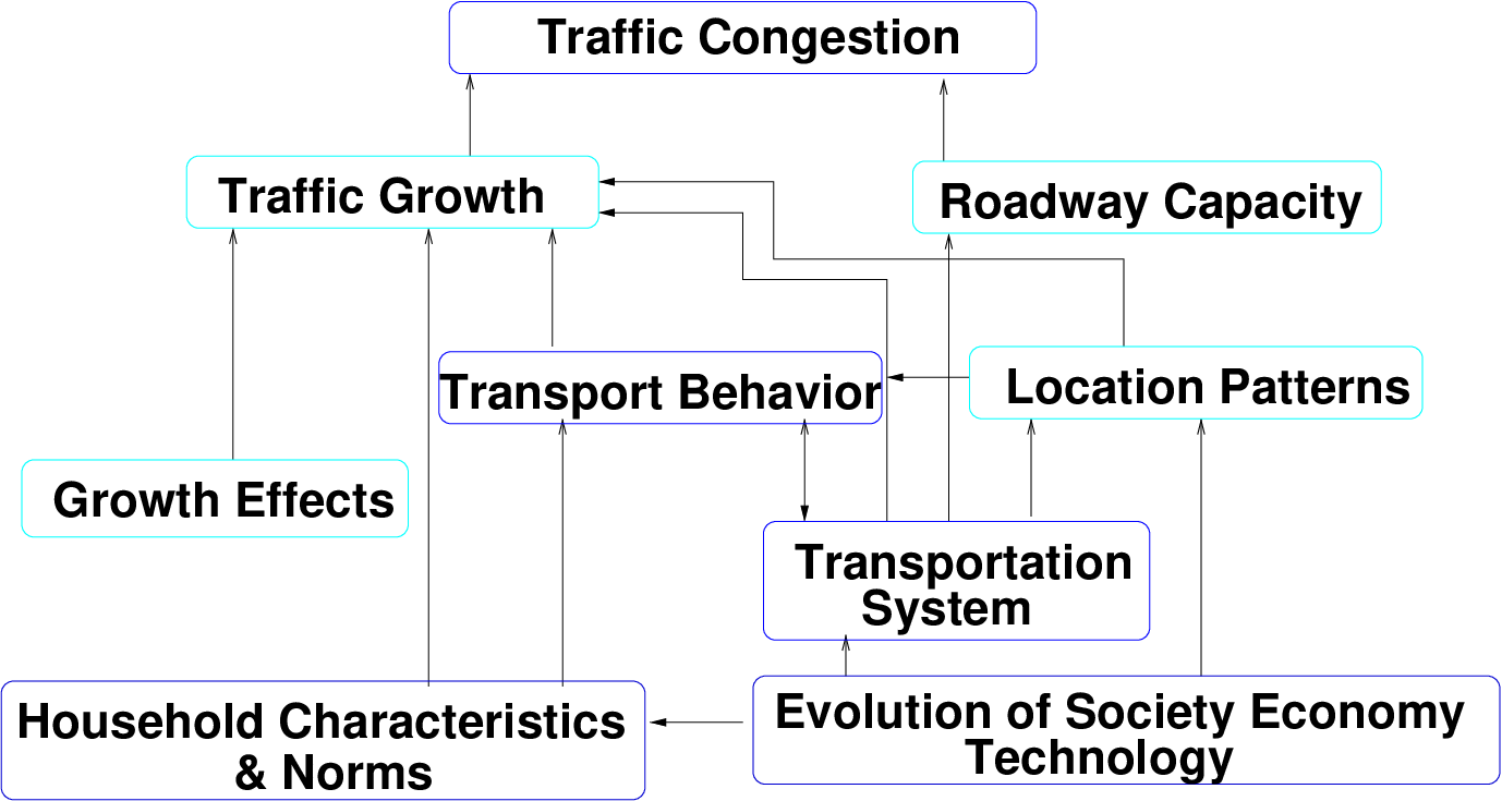
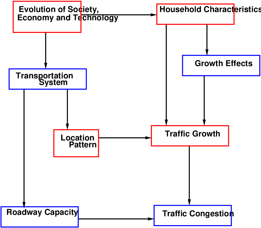
Figure 1: Generation of traffic congestion
Transportation system consists of a group of activities as well as entities interacting with each other to achieve the goal of transporting people or goods from one place to another. Hence, the system has to meet the perceived social and economical needs of the users. As these needs change, the transportation system itself evolves and problems occur as it becomes inadequate to serve the public interest. One of the negative impacts of any transportation system is traffic congestion. Traffic congestion occurs wherever demand exceeds the capacity of the transportation system. This lecture gives an overview of how congestion is generated, how it can be measured or quantified; and also the various countermeasures to be taken in order to counteract congestion. Adequate performance measures are needed in order to quantify congestion in a transportation system. Quality of service measures indicates the degree of traveller satisfaction with system performance and this is covered under traveller perception. Several measures have been taken in order to counteract congestion. They are basically classified into supply and demand measures. An overview of all these aspects of congestion is dealt with in this lecture.
The flow chart in Fig. 1 shows how traffic congestion is generated in a transportation system. With the evolution of society, economy and technology, the household characteristics as well as the transportation system gets affected. The change in transport system causes a change in transport behaviour and locational pattern of the system. The change in household characteristics, transport behaviour, locational pattern, and other growth effects result in the growth of traffic. But the change or improvement in road capacity is only as the result of change in the transportation system and hence finally a situation arises where the traffic demand is greater than the capacity of the roadway. This situation is called traffic congestion.
Congestion has a large number of ill effects on drivers, environment, health and the economy in the following ways.
The summation of all these effects yields a considerable loss for the society and the economy of an urban area
A system is said to be congested when the demand exceeds the capacity of the section. Traffic congestion can be defined in the following two ways:
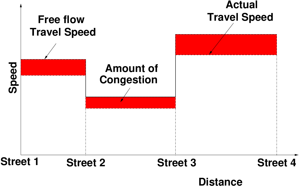
Fig. 2 shows the definition of congestion. The solid line represents the travel speed under free-flow conditions and the dotted line represents the actual travel speed. During congestion, the vehicles will be travelling at a speed less than their free flow speed. The shaded area in between these two lines represents the amount of congestion.
Traffic congestion may be of two types:
Congestion has to be measured or quantified in order to suggest suitable counter measures and their evaluation. Congestion information can be used in a variety of policy, planning and operational situations. It may be used by public agencies in assessing facility or system adequacy, identifying problems, calibrating models, developing and assessing improvements, formulating programs policies and priorities. It may be used by private sector in making locational or investment decisions. It may be used by general public and media in assessing traveler’s satisfaction.
Performance measure of a congested roadway can be done using the following four components:
Duration of congestion is the amount of time the congestion affects the travel system. The peak hour has now extended to peak period in many corridors. Measures that can quantify congestion include:
Duration of congestion is the sum of length of each analysis sub period for which the demand exceeds capacity. This component measures the performance of a particular road in handling traffic efficiently i,e.,with the increase in the duration of congestion, poorer will be the performance of the transportation system. The maximum duration on any link indicates the amount of time before congestion is completely cleared from the corridor. Duration of congestion can be computed for a corridor using the following equation: For corridor analysis,
 | (1) |
where, H is the duration of congestion (hours), N is the number of analysis sub periods for which v∕c > 1, and T is the duration of analysis sub-period (hours). For area wide analysis,
 | (2) |
where, Hi is the duration of congestion for link i (hours), T is the duration of analysis period (hours), r is the ratio of peak demand to peak demand rate, vi is the vehicle demand on link i (veh/hr), and ci is the capacity of link i (veh/hr).
Extent of congestion is described by estimating the number of people or vehicles affected by congestion and by the geographic distribution of congestion. These measures include:
Performance measures of extent of congestion can be computed from sum of length of queuing on each segment. Segments in which queue overflows the capacity are also identified. This is useful for ramp metering analysis. To compute queue length, average density of vehicles in a queue need to be known. The default values suggested by HCM 2000 are given in Table 1.
| Subsystem | Storage density | Spacing |
| (veh/km/lane) | (m) | |
| Free-way | 75 | 13.3 |
| Two lane highway | 130 | 7.5 |
| Urban street | 130 | 7.5 |
Queue length can be found out using the equation:
 | (3) |
where; QLi is the queue length (meter), v is the segment demand (veh/hour), c is the segment capacity (veh/hour), N is the number of lanes, ds is the storage density (veh/meter/lane), and T is the duration of analysis period (hour). If v < c, Qi=0 The equation for queue length is similar for both corridor and area-wide analysis.
Consider a road segment of 6 lanes with a capacity of 2400 veh/hr/lane. It is observed that the storage density is 75 veh/meter and the segment demand is found to be 2800 veh/hr/lane. Given that the duration of analysis sub period is 2 hrs calculate the queue length that is formed due to congestion.
Solution The queue length of a particular road segment is given by,
 | (4) |
It is given that Number of lanes, N=6, Duration of analysis sub period, T= 2 hrs, Segment Capacity=c=2400 veh/hr/lane, Segment Demand=v=2800 veh/hr/lane, Storage Density=ds=75 veh/meter. Now,the queue length can be calculated by using the above formula as follows: QL = 2 * (2800 - 2400) * 6∕(6 * 75) = 10.667mts Therefore, the extent of congestion in terms of queue length is 10.667mts
Intensity of congestion marks the severity of congestion. It is used to differentiate between levels of congestion on transport system and to define total amount of congestion. It is measured in terms of:
Intensity in terms of delay is given by,
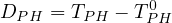 | (5) |
where, DPH is the person hours of delay, TPH is the person hours of travel under actual conditions, and TPH0 is the person hours of travel under free flow conditions. The TPH is given by:
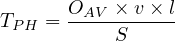 | (6) |
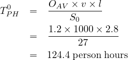
where, OAV is the average vehicle occupancy, v is the vehicle demand (veh), l is the length of link (km), and S is the mean speed of link (km/hr). The TPH is given by:
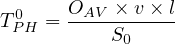 | (7) |
where, OAV is the average vehicle occupancy, v is the vehicle demand (veh), l is the length of link (km), and S0 is the free flow speed on the link (km/hr)
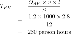
On a 2.8 km long link of road, it was found that the demand is 1000 Vehicles/hour mean
speed of the link is 12 km/hr, and the free flow speed is 27 km/hr. Assuming that the average
vehicle occupancy is 1.2 person/vehicle, calculate the congestion intensity in terms of total
person hours of delay.
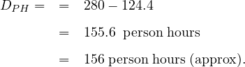
Solution: Given data: Length of the link=l=2.8 km, Vehicle demand=v=1000 veh, Mean Speed of the link=S=12 km/hr, Free flow speed on the link=So=27 km/hr, and Average Vehicle Occupancy=AVO=1.2 person/veh. Person hours of delay is given as

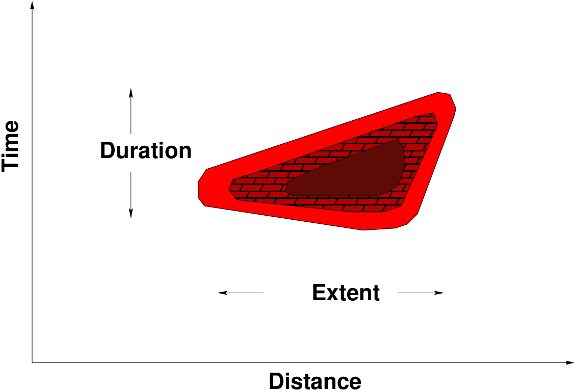
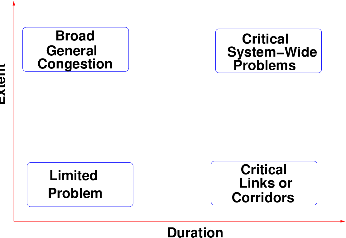
The variation in extent and duration of congestion indicates different problems requiring different solutions. Small delay and extent indicates limited problem, small delay for large extent indicates general congestion, great delay for small extent indicates critical links and great delay for large extent indicates critical system-wide problem. Fig. 3 also illustrates the relationship between duration, extent and intensity The extent of congestion is seen on the x-axis, the duration on the y-axis. The intensity is shown in the shading. Based on the extent and duration the congestion can be classified into four types as shown in Fig.4.
Fig.3 indicates a time distance graph with the shaded area indicating congestion in individual road segments for discrete time periods. The figure shows the relationship between duration, extent, and intensity.
The product of extent and duration indicates the intensity, or magnitude of the congestion problem.
Reliability is a measure of a driver’s ability to accurately predict and plan for a certain travel time. The more unexpected events that occur on a roadway, the less reliable it is. Non recurrent congestion has a bigger impact on the reliability of the roadway relative to concurrent congestion. In other words, Travel-time reliability is defined as the level of consistency in travel conditions over time and is measured by describing the distribution of travel times that occur over a substantial period of time. Reliability is an important component of roadway performance and perhaps more importantly, of motorist’s perceptions of roadway performance. The importance of measuring and managing reliability in reducing congestion is explained as follows.
Therefore, it is clear that reliability is the impact of non-recurrent congestion on transport system and it can be expressed as average travel rate or speed ± standard deviation or delay ± standard deviation.
Fully eradicating roadway congestion is neither an affordable, nor feasible goal in economically dynamic urban areas. However, much can be done to reduce its occurrence and to lessen its impacts on roadway users within large cities – congestion is a phenomenon that can be better and more effectively managed. There are many possible measures that can be deployed to “treat” or mitigate congestion.
Congestion countermeasures include supply measures and demand measures.,which will be discussed in detail in the next section. Other than these two measures, an additional longer-term tool used against traffic problems is land-use planning and policy. It has the potential
They add capacity to the system or make the system operate more efficiently. They focus on the transportation system. All measures in this category supply capacity so that demand is better satisfied and delays and queuing are lessened. Supply measures include
Demand measures focuses on motorists and travelers and attempt to modify their trip making behaviour. All the measures that are employed in this category aim to modify travel habits so that travel demand is considerably reduced or switch to other modes,other times or other locations that have more capacity to accommodate it. The demand measures include Congestion pricing, Parking pricing and Restrictions on vehicle ownership and use. Congestion pricing is the method in which users are charged on congested roads. This is discussed in detail in the next section. Parking pricing discourages use of private vehicles to specific areas. It includes heavy import duties, separate licensing requirement, heavy annual fees, expensive fuel prices, etc to restrain private vehicle acquisition and use. Heavy annual fees, strict periodic inspections and expensive fuel prices also restrict use of private vehicles. Intelligent Transportation systems (ITS) provide tools for implementation of both supply and demand congestion measures. Supply type ITS tools include early incident detection and resolution, optimized signal operation based on real time demand, freeway management with ramp metering, accident avoidance with variable message signs(VMS) warning of upcoming conditions(congestion, fog etc.,) and bus system coordination. Demand-type ITS include the provision of real-time traffic congestion information at various places for informed travel decisions.
Congestion pricing is a method of road user taxation, charging the users of congested roads according to the time spent or distance travelled on those roads. The principle behind congestion pricing is that those who cause congestion or use road in congested period should be charged, thus giving the road user the choice to make a journey or not.
Journey costs include private journey cost, congestion cost, environmental cost, and road maintenance cost. The benefit a road user obtains from the journey is the price he prepared to pay in order to make the journey. As the price gradually increases, a point will be reached when the trip maker considers it not worth performing or it is worth performing by other means. This is known as the critical price. At a cost less than this critical price, he enjoys a net benefit called as consumer surplus(es) and is given by:
 | (8) |
where, x is the amount the consumer is prepared to pay, and y is the amount he actually pays. The basics of congestion pricing involves demand function, private cost function as well as marginal cost function. These are explained below.
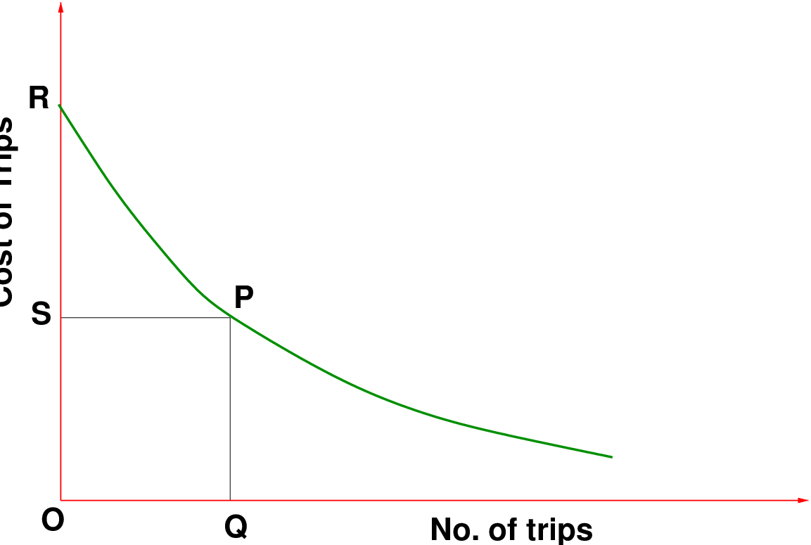
Fig. 5 shows the general form of a demand curve. In the figure, area QOSP indicates the absolute utility to trip maker and the area SRP indicates the net benefit.
Total private cost of a trip, is given by:
 | (9) |
where, a is the component proportional to distance, b is the component proportional to speed, and v is the speed of the vehicle (km/h). In the congested region, the speed of the vehicle can be expressed as,
 | (10) |
where, q is the flow in veh/hour, d and e are constants.
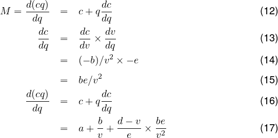
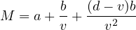
Marginal cost is the additional cost of adding one extra vehicle to the traffic stream. It reduces speed and causes congestion and results in increase in cost of overall journey. The total cost incurred by all vehicles in one hour(CT) is given by:
 | (11) |
Marginal cost is obtained by differentiating the total cost with respect to the flow(q) as shown in the following equations.
 | (18) |
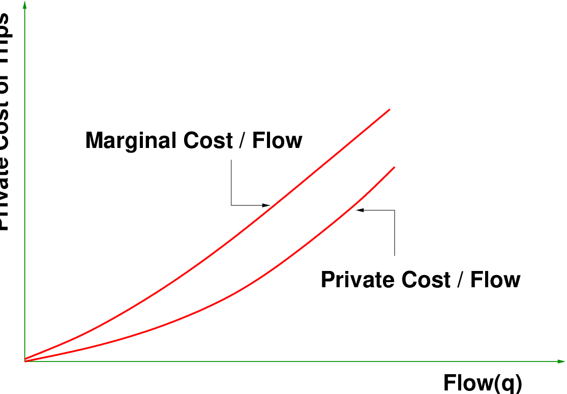
Fig. 6 shows the variation of marginal cost per flow as well as private cost per flow.
It is seen that the marginal cost will always be greater than the private cost, the increase representing the congestion cost.
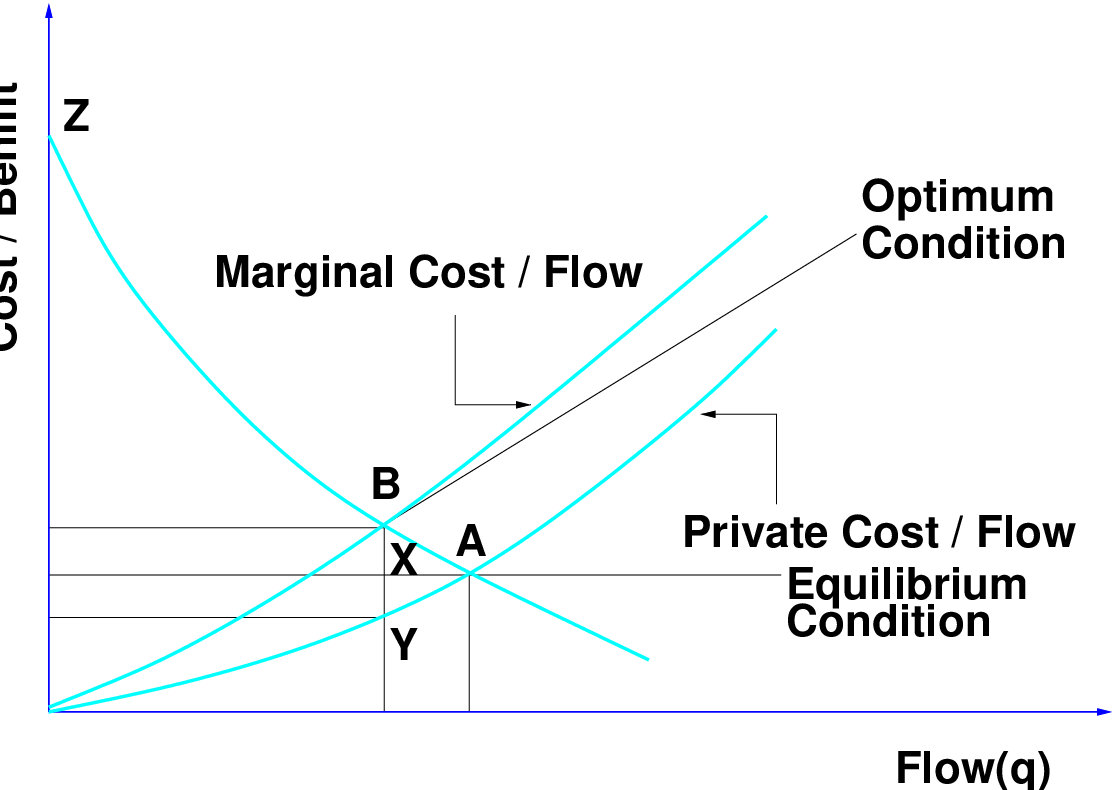
Superimposing the demand curve on the private cost/flow and marginal cost/flow curves, the position as shown in Fig. 7 is obtained. The intersection of the demand curve and the private costs curve at point A represents the equilibrium condition, obtained when travel decisions are based on private costs only. The intersection of the demand curve and the marginal costs curve at point B represents the optimum condition. At this point the flow Q0 corresponds to the cost C0 which is the marginal cost as well as the value of the trip to the trip maker. The net benefit under the two positions A and B are shown by the areas ACZ and BY CY Z respectively. If the conditions are shifted from point A to B, the net benefit due to change will be given by area CCyY X minus AXB. If the area CCyY X is greater than arc AXB, the net benefit will be positive. The shifting of conditions from point A to B can be brought about by imposing a road pricing charge BY. Under this scheme, the private vehicles continuing to use the roads will on an average be worse off in the first place because BY will always exceed the individual increase in benefits XY.
Vehicles are moving on a road at the rate of 500 vehicle/hour, at a velocity of 15 km/hr. Find the equation for marginal cost.
Solution: Private cost of the trip is given by,
Causes and effects of congestion along with various performance measures and with many other counter measures are discussed in detail considering the actual or technical definition of congestion. The congestion performance measures described are generalized measures. There are several other performance measures and indices. Advanced study on congestion can include improved measurement schemes and the combined travel demand modeling and route choice under congested conditions. With the implementation of all the counter measures traffic congestion, the most pronouncing problem of transportation may be reduced or controlled to certain extent. The principle and process of congestion pricing was also discussed with the help of certain graphs..
I wish to thank several of my students and staff of NPTEL for their contribution in this lecture. Specially, I wish to thank my student Ms. Anna Charly for his assistance in developing the lecture note, and my staff Mr. Rayan in typesetting the materials. I also appreciate your constructive feedback which may be sent to tvm@civil.iitb.ac.in
Prof. Tom V. Mathew
Department of Civil Engineering
Indian Institute of Technology Bombay, India
_________________________________________________________________________
Thursday 28 September 2023 11:39:58 AM IST