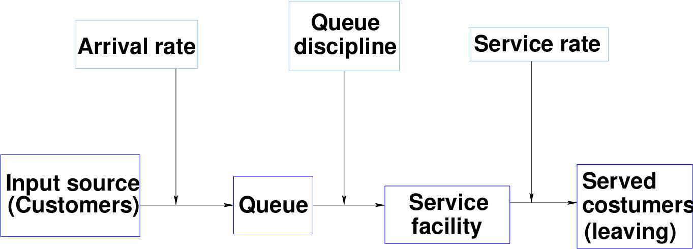
Figure 1: Components of a basic queuing system
One of the major issues in the analysis of any traffic system is the analysis of delay. Delay is a more subtle concept. It may be defined as the difference between the actual travel time on a given segment and some ideal travel time of that segment. This raises the question as to what is the ideal travel time. In practice, the ideal travel time chosen will depend on the situation; in general, however, there are two particular travel times that seem best suited as benchmarks for comparison with the actual performance of the system. These are the travel time under free flow conditions and travel time at capacity.
Most recent research has found that for highway systems, there is comparatively little difference between these two speeds. That being the case, the analysis of delay normally focuses on delay that results when demand exceeds its capacity; such delay is known as queuing delay, and may be studied by means of queuing theory. This theory involves the analysis of what is known as a queuing system, which is composed of a server; a stream of customers, who demand service; and a queue, or line of customers waiting to be served.
Figure 1 shows a schematic diagram illustrating the concept of a queuing system. Various components are discussed below.
These are explained in the following sections.
It is rate at which customers arrive at a service facility. It is expressed in flow (customers/hr or vehicles/hour in transportation scenario) or time headway (seconds/customer or seconds/vehicle in transportation scenario). If inter arrival time that is time headway (h) is known, the arrival rate can be found out from the equation:
 | (1) |
Mean arrival rate can be specified as a deterministic distribution or probabilistic distribution and sometimes demand or input are substituted for arrival.
It is the rate at which customers (vehicles in transportation scenario) depart from a transportation facility. It is expressed in flow (customers/hr or vehicles/hour in transportation scenario) or time headway (seconds/customer or seconds/vehicle in transportation scenario). If inter service time that is time headway (h) is known, the service rate can be found out from the equation:
 | (2) |
The number of servers that are being utilized should be specified and in the manner they work that is they work as parallel servers or series servers has to be specified.
Queue discipline is a parameter that explains how the customers arrive at a service facility. The various types of queue disciplines are
The following notation assumes that the system is in a steady-state condition (At a given time t):

Assume that λn is a constant λ for all n. It has been proved that in a steady-state queuing process, (λ may be considered as avg):

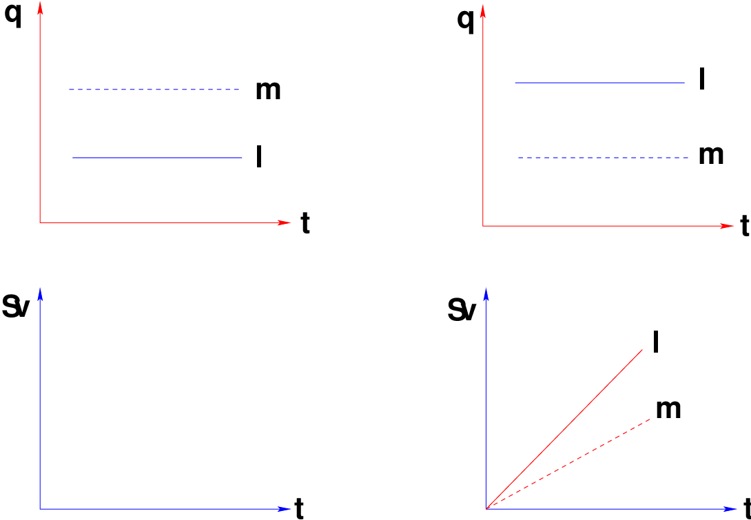
A variety of queuing patterns can be encountered and a classification of these patterns is proposed in this section. The classification scheme is based on how the arrival and service rates vary over time. In the following figures the top two graphs are drawn taking time as independent variable and volume of vehicles as dependant variable and the bottom two graphs are drawn taking time as independent variable and cumulative volume of vehicles as dependant variable.
In the left hand part of the Fig.2 arrival rate is less than service rate so no queuing is encountered and in the right hand part of the figure the arrival rate is higher than service rate, the queue has a never ending growth with a queue length equal to the product of time and the difference between the arrival and service rates.
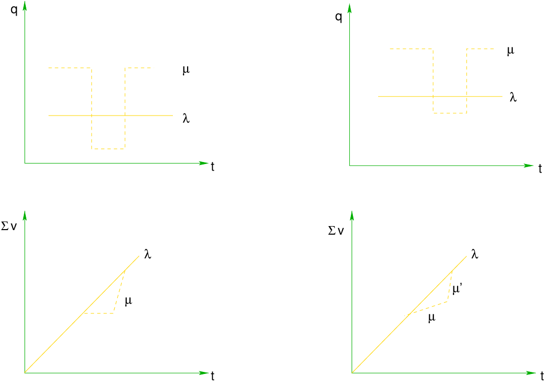
In the left hand of Fig. 3 the arrival rate is constant over time while the service rates vary over time. It should be noted that the service rate must be less than the arrival rate for some periods of time but greater than the arrival rate for other periods of time.
One of the examples of the left hand part of the figure is a signalized intersection and that of the right hand side part of the figure is an incident or an accident on the roads which causes a reduction in the service rate.
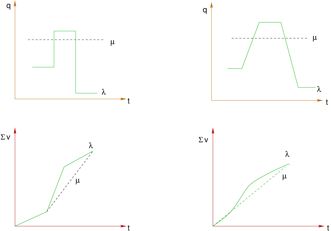
In the left part of Fig. 4 the arrival rate vary over time but service rate is constant. Both the left and right parts are examples of traffic variation over a day on a facility but the left hand side one is an approximation to make formulations and calculations simpler and the right hand side one considers all the transition periods during changes in arrival rates.
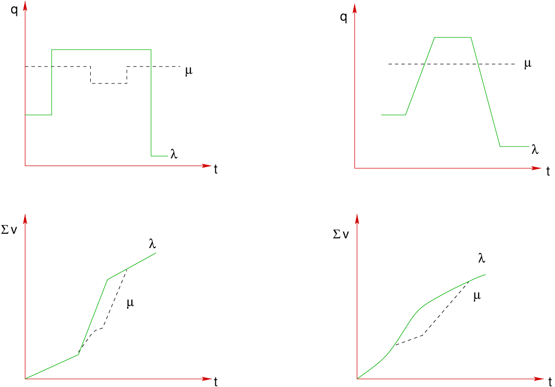
In the Fig.5 the arrival rate follows a square wave type and service rate follows inverted square wave type. The diagrams on the right side are an extension of the first one with transitional periods during changes in the arrival and service rates. These are more complex to analyzed using analytical methods so simulation is often employed particularly when sensitivity parameter is to be investigated.
There are various kinds of queuing models. These queuing models have a set of defined characteristics like some arrival and service distribution, queue discipline, etc. The queuing models are represented by using a notation which is discussed in the following section of queue notation.
In this model the arrival times and service rates follow Markovian distribution or exponential distribution which are probabilistic distributions, so this is an example of stochastic process. In this model there is only one server. The important results of this model are:


 = (1∕λ)
 =
= 
 =
=  ×
× =
= 
Vehicles arrive at a toll booth at an average rate of 300 per hour. Average waiting time at
the toll booth is 10s per vehicle. If both arrivals and departures are exponentially
distributed, what is the average number of vehicles in the system, average queue
length, the average delay per vehicle, the average time a vehicle is in the system?
Solution
Mean arrival rate λ = 300 vehicles/hr. Mean service rate μ =  vehicles/hr. Utilization
factor = traffic intensity = ρ =
vehicles/hr. Utilization
factor = traffic intensity = ρ =  =
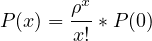
=  = 0.833. Percent of time the toll booth will be idle = P(0)
= P(X=0) = ρ0(1 - ρ) = (0.833)0(1 - 0.833) = 0.139(60min)=8.34 min. Average number of
vehicles in the system = E[X] =
= 0.833. Percent of time the toll booth will be idle = P(0)
= P(X=0) = ρ0(1 - ρ) = (0.833)0(1 - 0.833) = 0.139(60min)=8.34 min. Average number of
vehicles in the system = E[X] =  =4.98. Average number of vehicles in the queue
=E[Lq] =
=4.98. Average number of vehicles in the queue
=E[Lq] =  = 4.01. Average a vehicle spend in the system =E[T] =
  = 0.016 hr = 0.96
min = 57.6 sec. Average time a vehicle spends in the queue =E[Tq] =
= 0.016 hr = 0.96
min = 57.6 sec. Average time a vehicle spends in the queue =E[Tq] =  = 0.013hr = 0.83
min = 50 sec.
= 0.013hr = 0.83
min = 50 sec.
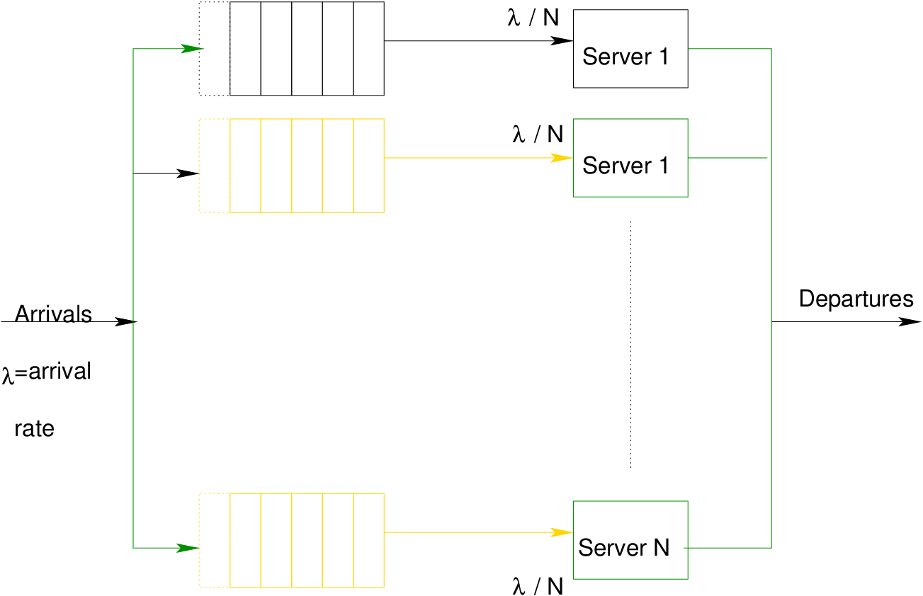
The difference between the earlier model and this model is the number of servers. This is a multi -server model with N number of servers whereas the earlier one was single server model. The assumptions stated in M/M/1 model are also assumed here.
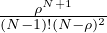
Here μ is the average service rate for N identical service counters in parallel. For x=0
![[ ]
N∑-1( ρx ρN ) -1
P (0) = x! + (N--- 1)!(N---ρ)
x=0](web20x.png) | (3) |
The probability of x number of customers in the system is given by P(x). For 1 ≤ x ≤ N
 | (4) |
For x > N
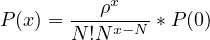 | (5) |
The average number of customers in the system is
![E [X ] = ρ+ [----ρN+1------]P (0)
(N - 1)!(N - ρ)2](web23x.png) | (6) |
The average queue length
![E[Lq] = [(N---1ρ)N!+(N1--ρ)2]P(0)](web24x.png) | (7) |
The expected time in the system
![E [X ]
E [T] =--λ--](web25x.png) | (8) |
The expected time in the queue
![E [Lq]
E[Tq] =--λ--](web26x.png) | (9) |
Consider the earlier problem as a multi-server problem with two servers in parallel.
Solution
Average arrival rate = λ = 300 vehicles/hr. Average service rate = μ =  vehicles/hr.
Utilization factor = traffic intensity = ρ =
vehicles/hr.
Utilization factor = traffic intensity = ρ =  =
=  = 0.833.
![[ ]
N∑-1 (ρx ρN ) -1
P(0) = x! + (N---1)!(N---ρ)
x=0
= 0.92(60) = 55.2min](web30x.png)
 ]P(0) = 1.22. The
average number of customers in the queue = Lq = E[Lq] = [
]P(0) = 1.22. The
average number of customers in the queue = Lq = E[Lq] = [ ]P(0)= 0.387.
Expected time in the system =W =
]P(0)= 0.387.
Expected time in the system =W = ![E-[Xλ]](web33x.png) = 0.004 hr = 14 sec. The expected time in the queue
=Wq =
= 0.004 hr = 14 sec. The expected time in the queue
=Wq =  = 0.00129 hr = 4.64 sec.
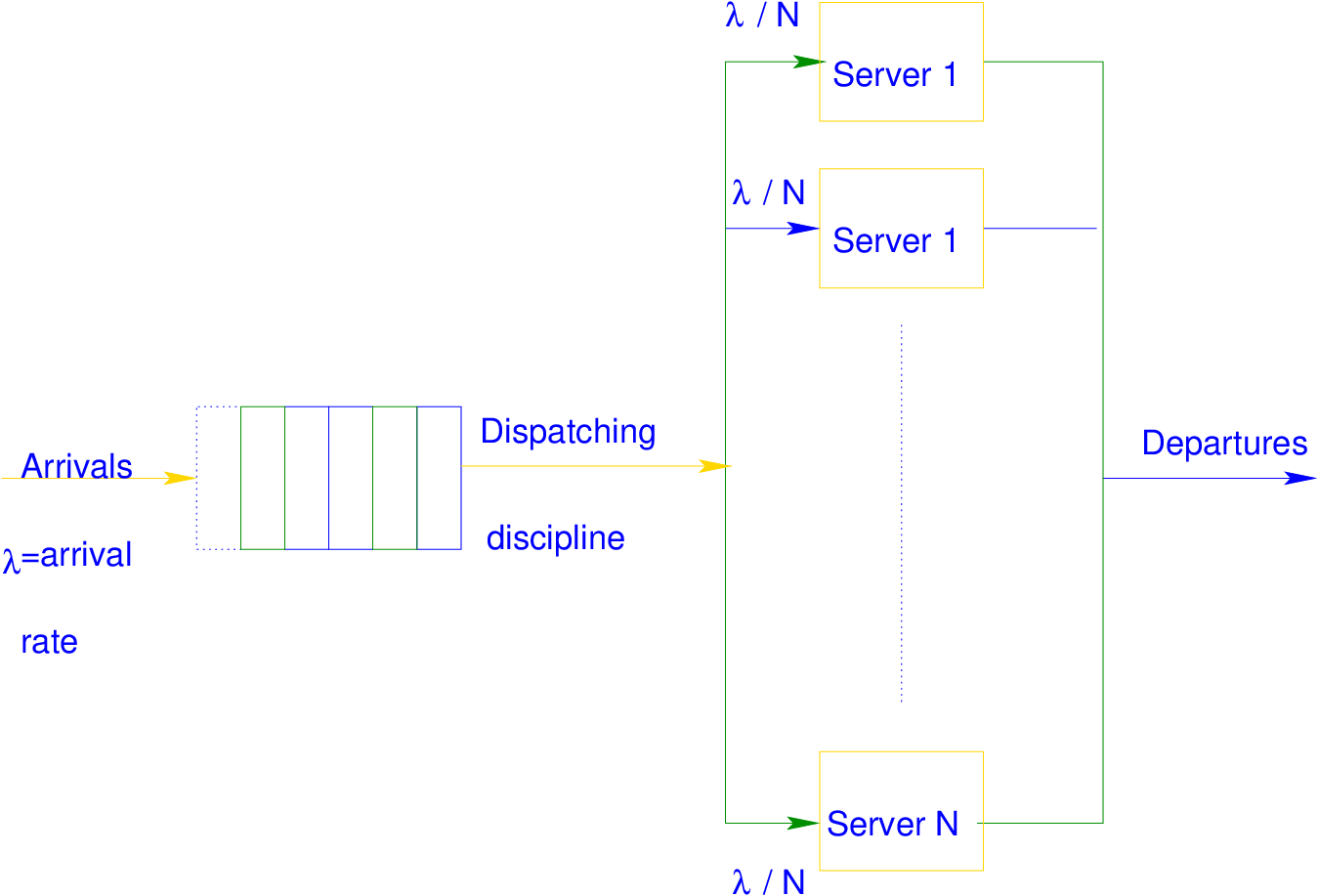
In this model there are N numbers of identical independent parallel servers which receive
customers from a same source but in different parallel queues (Compare to M/M/N model. It
has only one queue) each one receiving customers at a rate of  . Fig. 7 shows how a typical
multiple single servers’ model looks like.
. Fig. 7 shows how a typical
multiple single servers’ model looks like.
Consider the problem 1 as a multiple single server’s model with two servers which work independently with each one receiving half the arrival rate that is 150 vehicles/hr.
Solution
Mean arrival rate = λ = 150 vehicles/hr. Mean service rate =μ =  vehicles/hr. Utilization
factor = traffic intensity = ρ =
vehicles/hr. Utilization
factor = traffic intensity = ρ =  =
=  = 0.416. The percent of time the toll booth
will be idle = P(0) = P(X=0) = (0.416)0(1 - 0.416) = 0.584(60min)=35.04 min. The
average number of vehicles in the system = E[X] =
= 0.416. The percent of time the toll booth
will be idle = P(0) = P(X=0) = (0.416)0(1 - 0.416) = 0.584(60min)=35.04 min. The
average number of vehicles in the system = E[X] =  = 0.712. The average number
of vehicles in the queue =Lq =
= 0.712. The average number
of vehicles in the queue =Lq =  = 0.296. The average a vehicle spend in the
system =E[T] = W =
= 0.296. The average a vehicle spend in the
system =E[T] = W =  = 0.0047 hr = 0.285 min = 17.14 sec. The average time a
vehicle spends in the queue =E[Tq] = Wq =
= 0.0047 hr = 0.285 min = 17.14 sec. The average time a
vehicle spends in the queue =E[Tq] = Wq =  = 0.0022hr = 0.13 min = 8.05
sec
= 0.0022hr = 0.13 min = 8.05
sec
| M/M/1 model | M/M/2 model | Multiple single | |
| server model | |||
| Idle time of toll | 8.34 | 55.2 | 35.04 |
| booths(minutes) | |||
| Number of vehicles | 4.98 | 1.22 | 0.712 |
| in the system(units) | |||
| Number of vehicles | 4.01 | 0.387 | 0.296 |
| in the queue(units) | |||
| Average waiting time | 57.6 | 14 | 17.14 |
| in system(seconds) | |||
| Average waiting time | 50 | 4.64 | 8.05 |
| in queue(seconds) | |||
From the Table 1 by providing 2 servers the queue length reduced from 4.01 to 0.387 and the average waiting time of the vehicles came down from 50 sec to 4.64 sec, but at the expense of having either one or both of the toll booths idle 92% of the time as compared to 13.9% of the time for the single-server situation. Thus there exists a trade-off between the customers’ convenience and the cost of running the system.
In this model the arrival and service rates are deterministic that is the arrival and service times of each vehicle are known.
Morning peak traffic upstream of a toll booth is given in the table 2. The toll plaza consists of three booths, each of which can handle an average of one vehicle every 8 seconds. Determine the maximum queue, the longest delay to an individual vehicle.
| Time period | 10 min volume |
| 7.00-7.10 | 200 |
| 7.10-7.20 | 400 |
| 7.20-7.30 | 500 |
| 7.30-7.40 | 250 |
| 7.40-7.50 | 200 |
| 7.50-8.00 | 150 |
Solution The arrival volume is given in the table. Service rate is given as 8 seconds per vehicle. This implies for 10 min, 75 vehicles can be served by each server. It is given there are 3 servers. Hence 225 vehicles can be served by 3 servers in 10 min. In the first 10 min only 200 vehicles arrive which are served so the service rate for rest 50 min is 225 veh/10 min as there is a queue for the rest period. The solution to the problem is showed in the table 3 following. The cumulative arrivals and services are calculated in columns 3 and 5. Queue length at the end of any 10 min interval is got by simply subtracting column 5 from column 3 and is recorded in column 6. Maximum of the column 6 is maximum queue length for the study period which is 300 vehicles. The service rate has been found out as 225 vehicles per hour. From proportioning we get the time required for each queue length to be served and as 475 vehicles is the max queue length, the max delay is corresponding to this queue. Therefore max delay is 21.11 min.
| Time | 10 min | Cum. | Service | Cumulative | Queue | Delay |
| period | flow (3) | rate(4) | service(5) | =(3)-(4) | (6) | |
| 7.00-7.10 | 200 | 200 | 200 | 200 | 0 | 0 |
| 7.10-7.20 | 400 | 600 | 225 | 425 | 175 | 7.78 |
| 7.20-7.30 | 500 | 1100 | 225 | 650 | 450 | 20.00 |
| 7.30-7.40 | 250 | 1350 | 225 | 875 | 475 | 21.11 |
| 7.40-7.50 | 200 | 1550 | 225 | 1100 | 450 | 20.00 |
| 7.50-8.00 | 150 | 1700 | 225 | 1325 | 375 | 16.67 |
The queuing models often assume infinite numbers of customers, infinite queue capacity, or no bounds on inter-arrival or service times, when it is quite apparent that these bounds must exist in reality. Often, although the bounds do exist, they can be safely ignored because the differences between the real-world and theory is not statistically significant, as the probability that such boundary situations might occur is remote compared to the expected normal situation. Furthermore, several studies show the robustness of queuing models outside their assumptions. In other cases the theoretical solution may either prove intractable or insufficiently informative to be useful. Alternative means of analysis have thus been devised in order to provide some insight into problems that do not fall under the scope of queuing theory, although they are often scenario-specific because they generally consist of computer simulations or analysis of experimental data.
I wish to thank several of my students and staff of NPTEL for their contribution in this lecture. Specially, I wish to thank my students Mr. Pradham Kumar and Dillip Rout for their assistance in developing the lecture note, and my staff Mr. Rayan in typesetting the materials. I also appreciate your constructive feedback which may be sent to tvm@civil.iitb.ac.in
Prof. Tom V. Mathew
Department of Civil Engineering
Indian Institute of Technology Bombay, India
_________________________________________________________________________
Thursday 28 September 2023 11:40:12 AM IST