Non-Liner Programming
Lecture Notes in Transportation Systems Engineering
1 Optimization is the act of obtaining the best result under given circumstances. It is the process of finding
the condtions that give maximum or minimum value of a function. The general form of the optimization
problem will be to find \(\bar {x}\) that
\begin {eqnarray*} \mathrm {Minimize} & f(\bar {x}) & \\ \mathrm {subjected~to} \\ g_j(\bar {x}) & \le & 0\\ h_j(\bar {x}) & = & 0. \end {eqnarray*}
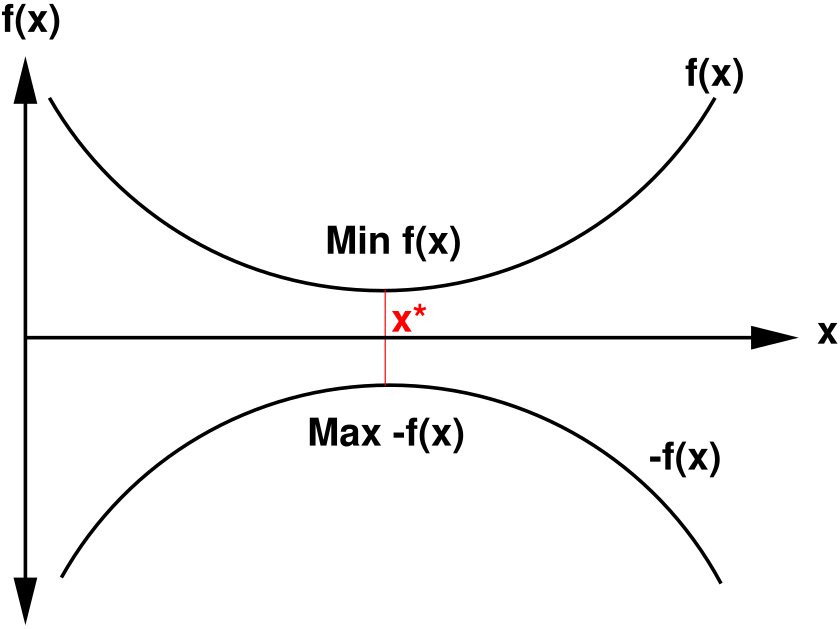
where \(\bar {x}\) is the decision variable. Figure 1 shows the concept of optimization which is to find the
minimum or maximum of a function. Since Minimizing \(f(x)\) is same as maximizing \(-f(x)\) we shall follow the former
notation. The optimum solution is indicated by \(\bar {x}^*\)
Figure 1: The concept of optimisation
2
2.1
2.1.1 Determin the convexity of the following function:
\begin {eqnarray*} f(x_1,x_2)=(x_1-x_2)^2 , \end {eqnarray*}
2.1.2 Determin the convexity of the following functions:
\begin {eqnarray*} f(\bar {x})&=&x_1-2x_1x_2+x_2^2\\ f(\bar {x})&=&x_1^2+x_2^2+x_3^2-x_1x_2+x_2x_3-x_1x_3\\ f(x)&=&4x_1^4+2x_1^2-5x_1 \end {eqnarray*}
3
3.1
3.1.1 Solve the function and iterpret the results(s):
\begin {eqnarray*} f(x)=12x^5-45x^4+40x^3+5. \end {eqnarray*}
3.1.2 Solve the following functions and iterpret the results(s):
\begin {eqnarray*} f(x)&=&(x-7)^2,\\ f(x)&=&x(x-1.5),\\ f(x)&=&-3x^2+21.6x+1. \end {eqnarray*}
3.2
3.2.1 Solve the function and iterpret the results(s):
\begin {eqnarray*} f(\bar {x})=x_1^3+x_2^3+2x_1^2+4x_2^2+6. \end {eqnarray*}
3.2.2 Solve the following functions and iterpret the results(s):
\begin {eqnarray*} f(\bar {x})&=&(x_1-10)^2+(x_2-10)^2. \end {eqnarray*}
3.3
3.3.1 Solve the following constrained program:
\begin {eqnarray*} \mathrm {Min:~} f(\bar {x})&=&x_1^2+2x_2,\\ \mathrm {st:~} g(\bar {x})&=&x_1^2+x_2^2=1. \end {eqnarray*}
3.3.2 Solve the following constrained program:
\begin {eqnarray*} \mathrm {Min:~} f(x,y)&=&kx^{-1}y^{-2},\\ \mathrm {st:~} g(x,y)&=&x^2+y^2=a^2. \end {eqnarray*}
Solve the following constrained program:
\begin {eqnarray*} \mathrm {Min:~} f(x,y,z)&=&3x^2+4y^2+5z^2,\\ \mathrm {st:~} g(x,y,z)&=&x+y+z=10. \end {eqnarray*}
3.4
3.4.1 Solve the following constrained program:
\begin {eqnarray*} \mathrm {Min:~} f(\bar {x})&=&x_1^2-x_2,\\ \mathrm {st:~} x_1+x_2&=&6,\\ x_1&\ge &1,\\ x_1^2+x_2^2&\le &26. \end {eqnarray*}
3.4.2 Solve the following constrained program:
\begin {eqnarray*} \mathrm {Max:~} f(\bar {x})&=&\log (x_1+1)+x_2,\\ \mathrm {st:~} 2x_1+x_2&\le &3,\\ x_1,x_2&\ge &0. \end {eqnarray*}
Solve the following constrained program:
\begin {eqnarray*} \mathrm {Min:~} f(x,y,z)&=&3x^2+4y^2+5z^2,\\ \mathrm {st:~} g(x,y,z)&=&x+y+z=10. \end {eqnarray*}
4
4.1
4.1.1 Solve the following unconstrained one dimentional problem:
\begin {eqnarray*} \mathrm {Max:~} f(x)&=&12x-3x^4-2x^6. \end {eqnarray*}
4.1.2 Solve the following unconstrained one dimentional problems
\begin {eqnarray*} \mathrm {Min:~} f(x)&=&x(x-1.5), ~~[0-1];\\ \mathrm {Min:~} f(x)&=&0.65-\frac {0.75}{1+x^2}-0.65x\tan ^{-1}\left ({\frac {1}{x}}\right ),\\&& ~~[0-3];\\ \mathrm {Max:~} f(x)&=&-3x^2+21.6x+1, ~~[0-25]. \end {eqnarray*}
4.2
4.2.1 Solve the following unconstrained multi-variable problem:
\begin {eqnarray*} \mathrm {Max:~} f(\bar {x})=2x_1x_2+2x_2-x_1^2-2x_2^2, ~~ \bar {x}^0=(0,0). \end {eqnarray*}
4.2.2 Solve the following unconstrained multi-variable problems:
\begin {eqnarray*} \mathrm {Min:~} f(\bar {x})=4x_1^2-4x_1x_2+2x_2^2, ~~ \bar {x}^0=(2,3). \end {eqnarray*}
4.3
4.3.1 It is type of sequential approximation algorithm. This is applicable when the objective function is non
liner and the constraints are all liner. It uses a linear approximation of the objetive function and solve by
any classical linear programming algorithm.
Given a feasible trail solution (\(\bar {x}=\bar {x}^1\)), then the linear approximation used for the objective function is the
first order Taylor series expansion of \(f(\bar {x})\) around \(\bar {x}=\bar {x}^1\). Thus
\begin {eqnarray} f(\bar {x})&=&f(\bar {x}^1)+\sum ^n_{j=1}\frac {\partial f(\bar {x}^1)}{\partial x_j}(x_j-x_j^1)\\ &=&f(\bar {x}^1)-\sum ^n_{j=1}\frac {\partial f(\bar {x}^1)}{\partial x_j}x_j^1+\sum ^n_{j=1}\frac {\partial f(\bar {x}^1)}{\partial x_j}x_j\\ &=&f(\bar {x}^1)-\sum ^n_{j=1}\frac {\partial f(\bar {x}^1)}{\partial x_j}x_j^1+g(\bar {x}) \end {eqnarray}
Since the first and second term of \(f(x)\) is constant, optimzing \(f(x)\) is same as optimizing \(g(x)\). Therefore, the
equivalent linear form of \(f(x)\) is \(g(x)\), that is,
\begin {eqnarray} g(\bar {x})&=&\sum ^n_{j=1}\frac {\partial f(\bar {x}^1)}{\partial x_j}x_j\\ &=&\sum ^n_{j=1}c_j~x_j,~\mathrm {where~}c_j=\left | \frac {\partial f(\bar {x})}{\partial x_j}\right |_{\bar {x}=\bar {x}^1} \end {eqnarray}
Frank-Wolfe Algorithm
Set \(k\)=0, find initital solution \(\bar {x}^k\)
Set \(k=k+1\) compute \(c_j=\left | \frac {\partial f(\bar {x})}{\partial x_j}\right |_{\bar {x}=\bar {x}^{k-1}}~\forall j=1,2,\dots ,n\)
Find optimum solution \(x^k_{LP}\) for the following LP
\begin {eqnarray} \mathrm {Max:~} g(\bar {x})&=&c_j~x_j,\nonumber \\ \mathrm {s.t.~~} A\bar {x}&\leq &\bar {b},\nonumber \\ \bar {x}&\geq &0.\nonumber \end {eqnarray}
For the variable \(t,~0\leq t \leq 1\) set
\begin {eqnarray} h(t)=f(\bar {x}^k)&\mathrm {where}&\bar {x}^k=\bar {x}^{k-1}+t\left [\bar {x}^k_{LP} - \bar {x}^{k-1} \right ]\nonumber \end {eqnarray}
Find \(t^*\) that maximizes \(h(t)\) in the interval \(0\leq t\leq 1\) and compute the next point by
\begin {eqnarray} \bar {x}^k=\bar {x}^{k-1}+t^*\left [\bar {x}^k_{LP} - \bar {x}^{k-1} \right ] \end {eqnarray}
If the error \(\epsilon \geq |\bar {x}^k - \bar {x}^{k-1}|\) go to step 2, else STOP.
Note that in step 1 use LP to get a feasible initital solution. Also in step 5 use any one dimentional search
(either numerical or classical) to maximize the function \(h(t)\).
4.3.2 Solve the following program by frank-wolfe alogorithm:
\begin {eqnarray*} \mathrm {Max:~} f(\bar {x})&=&5x_1-x_1^2+8x_2-2x_2^2,\\ \mathrm {st:~} 3x_1+2x_2&\le &6,\\ x_1,x_2&\ge &0. \end {eqnarray*}
Solution
Set \(k=0\), and assume \(\bar {x}^0=(0,0)\)
compute \(c_1\) and \(c_2\) as follows:
\begin {eqnarray*} c_1&=&\left .\frac {\partial f}{\partial x_1}\right |_{x_{1=0}}=5-2x_1=5\\ c_2&=&\left .\frac {\partial f}{\partial x_2}\right |_{x_{2=0}}=8-4x_2=8\\ g(x_1,x_2)&=&5x_1+8x_2 \end {eqnarray*}
Solve the following LP:
\begin {eqnarray} \mathrm {Max:~} g(\bar {x})&=&5x_1+8x_2,\nonumber \\ \mathrm {s.t.~~} 3x_1+2x_2&\leq &6,\nonumber \\ x_1,x_2&\geq &0.\nonumber \end {eqnarray}
Solving graphically, \(\bar {x}^*=(0,3)\)
Setting \(\bar {x}^k=(0,0)+t[(0,3)-(0,0)]=(0,3t)\)
Therefore, \(h(t)=f(0,3t)=(5\times 0)+(0)^2+8(3t)-2(3t)^2=24t-18t^2\)
Solving, \(\frac {\partial {h(t)}}{\partial t}=24-36t=0, \rightarrow t^*=\frac {24}{36}=\frac {2}{3}\)
Therfore, the new trail solution is \(x_k=(0,[3\times \frac {2}{3}])=(0,2)\)
k \(x^{(k-1)}\) \((c_1,c_2)\) \(x^k_{LP}\) x(t) h(t) \(t^*\) \(x^k\)
0 0, 0 5, 8 0, 3 0, 3t 24t-18t\(^2\) 2/3 0, 2
4.3.3 Solve the following program by frank-wolfe alogorithm:
\begin {eqnarray*} \mathrm {Min:~} f(\bar {x})&=&(x_1-x_2)^2+x_2,\\ \mathrm {st:~} x_1+x_2&\ge &1,\\ x_1+2x_2&\le &3,\\ x_1,x_2&\ge &0. \end {eqnarray*}
4.3.4 Solve the following program by frank-wolfe alogorithm:
\begin {eqnarray*} \mathrm {Max:~} f(\bar {x})&=&3x_1+4x_2-x_1^3-x_2^3,\\ \mathrm {st:~} x_1+x_2&\le &1,\\ x_1,x_2&\ge &0. \end {eqnarray*}
4.3.5 Solve the following program by frank-wolfe alogorithm:
\begin {eqnarray*} \mathrm {Max:~} f(\bar {x})&=&4x_1-x_1^4+2x_2-x_2^2,\\ \mathrm {st:~} 4x_1+2x_2&\le &5,\\ x_1,x_2&\ge &0. \end {eqnarray*}
4.3.6 Solve the following program by inner penalty function method:
\begin {eqnarray*} \mathrm {Min:~} f(\bar {x})&=&\frac {(x_1+1)^3}{3}+x_2,\\ \mathrm {st:~} -x_1+1&\le &0,\\ -x_2&\le &0.\\ \end {eqnarray*}
4.3.7 Solve the following program by exterior penalty function method:
\begin {eqnarray*} \mathrm {Min:~} f(\bar {x})&=&\frac {(x_1+1)^3}{3}+x_2,\\ \mathrm {st:~} -x_1+1&\le &0,\\ -x_2&\le &0.\\ \end {eqnarray*}
Not Available
K Deb. Optimization for engineering design: Algorithms and Examples . Prentice Hall, India,
1998.
F S Hillier and G J Lieberman. Introduction to operations research . McGraw Hill, Inc., 2001.
Singiresu S Rao. Engineering optimization: Theory and practice . New Age International,
New Delhi, India, 1996.
A Ravindran, D T Philips, and J J Solberg. Operations research: Principles and practice .
John Wiley and Sons, 1987.
H A Taha. Operations research: An introduction . Prentice-Hall, India, 1997.
I wish to thank several of my students and staff of NPTEL for their contribution in this lecture. I
also appreciate your constructive feedback which may be sent to tvm@civil.iitb.ac.in . Prof.
Tom V. Mathew, Department of Civil engineering, Indian Instiute of Technology Bombay,
India.