Objective: a clear statement of the basic principles of underlying the theory and application
of network flows in transportation.
Applicable to road traffic, rail, shipping, and airline network.
Assist in transportation planning and traffic control applications.
Examples of network representation:
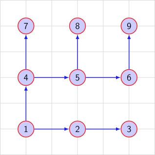
Road Network
Traffic Desire Network
2 Graphs: Definitions and Notations
2.1 Directed Graph
Directed graph [\(N\),\(L\)] is a set of \(N\) unordered elements and a set of \(L\) ordered pairs of elements of
\(N\).
Number of elements in \(N\) and \(L\) are \(n\) and \(l\) respectively.
\(N~(n_i, i=1, 2, \dots , n)\) is the set of node and \(L~(l_k(n_i,n_j),~n_i\in N,~n_j\in N, k=1,2,\dots ,l)\) is the set of links.
Here, we assume there is no parallel link.
If \(n_i=n_j\) then the link is a loop (nodes defining link may or may not be distinct).
It is common practice to call the nodes \(n_i\) and \(n_j\) defining the link \(l_k(n_i,n_j)\) as A node and B node
respectively.
Partial Graph of the directed graph [\(N\),\(L\)] is defined as [\(N\),\(L'\)] where \(L'\subseteq L\). This is obtained by deleting
links.
Sub Graph of the directed graph [\(N\),\(L\)] is defined as [\(N'\),\(L'\)] where \(N'\subseteq N\) and \(L'=\{(n_i,n_j)|(n_i,n_j)\in L, n_i\in N', n_j\in N'\}\). Obtained by deleting nodes
and attached links.
Complete Graph is graph with at least one link joining any two distinct nodes of \(N\), that is,
\(n_i\in N,~n_j\in N,~n_i\neq n_j,~ (n_i,n_j)\notin L \Rightarrow (n_j,n_i)\in L\).
Bipartite Graph is a graph in which the set of \(N\) nodes is divided into two complementary
set \(X,\bar {X}\), such that, \(X\cup \bar {X}=N\) and \(X\cap \bar {X}=\emptyset \) and \(L=\{(n_i,n_j)|n_i\in X,~n_j\in \bar {X}\}\)
If \(n_1, n_2 \dots n_r\) are distinct nodes, then the sequence \(n_1 (n_1, n_2) n_2 (n_2,n_3) n_3 \dots n_{r-1} (n_{r-1}, n_r) n_r\) defines a chain from origin node \(n_14\) to destination node \(n_r\). If \(n_1=n_r\) then
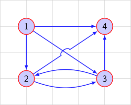
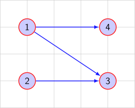
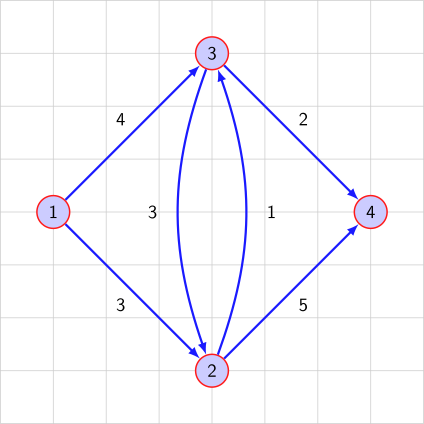
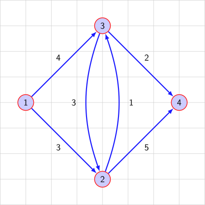
chain becomes a cycle. In figure 1 1 (1,2) 2 (2,3) 3 (3,4) 4 is a chain from node 1 to 4 while 2 (2,3) 3 (3,2)
2 is a cycle from 2 to 2.
2.3 Path and Mesh
If directions of links are not considered chain and cycle becomes path and mesh respectively. If \(n_1, n_2 \dots n_r\) are
distinct nodes \((n_i',n_{i+1}')\) are links, then a path from origin node \(n_1\) to destination node \(n_r\) is defined by the
sequence \(n_1 (n_1',n_2') n_2 \dots n_i (n_i',n_{i+1}') n_{i+1} \dots n_r)\) where either \(n_i'=n_i\) and \(n_{i+1}'=n_{i+1}\) (forward link) or \(n_i'=n_{i+1}\) and \(n_{i+1}'=n_i\) (reverse link). The path becomes a mesh if
\(n_1=n_r\).
2.4 Accessible and connected nodes
In a graph, n1 to nr is accessible if there exists a chain from n1 to nr and is connected if there exists a path
from n1 to nr. If n1 to nr is accessible, that does not imply nr to n1 is accessible, however, if n1 to nr is
connected, that does imply nr to n1 is connected.
A connected directed graph is a graph in which all nodes are connected.
2.5 Cut-Set
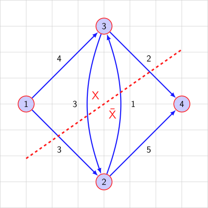
If the set of nodes N is partitioned into complementary sets \(X\) and \(\bar {X}\) then the sub set \(L\) defined by (\(X,\bar {X})=\{(i,j)| (i,j)\in L, i\in X, j\in \bar {X}\) is
called a cut set. Refer to the graph in figure 1: if \(X=\{1,2\}\) and \(\bar {X}=\{3,4\}\), then cut set (\(X, \bar {X}\))={(1,3), (1,4), (2,3),
(2,4)} and the cut set (\(\bar {X},X\))={(3,2)}. Cut set has several applications in transportation networks,
for example the road links crossing a screen lines and cordon lines can be modelled as cut
sets.
2.6 Undirected and mixed graphs
The undirected graph [\(N,L\)], the elements of \(L\) are unordered pair of elements of \(N\) and are denoted as (\(n_i,n_j\)) or (\(n_j,n_i\)).
Arrow heads are not required for their representation. Pedestrian link or two way streets are some
examples.
2.7 Tree and Arborescence
A tree denoted by [\(N,T\)] is a connected graph with no meshes (directions are ignored). A graph is a tree if and
only if every pair of distinct nodes is connected precisely one path. A spanning tree of a graph [\(N,L\)] is a tree [\(N,T\)]
which is a partial graph of [\(N,L\)], that is, \(T\subseteq L\) When directions are considered, then the tree which
consists of chains from home node to all other nodes is called and Arborescence. Hence, an
Arborescence is a directed graph in which, for a node \(n_r\) called as the root and any other node \(n_i\), there is
exactly one directed path from \(n_r\) to \(n_i\). Spanning tree has application in finding the shortest
path.
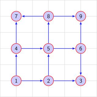
Figure 6: Directed Graph G (N, L)
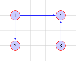
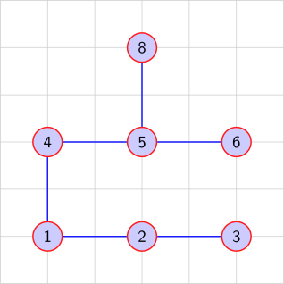
Figure 7: A Graph G’ (N’,T) which is a tree,
but not a spanning tree of G (N, L)
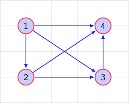
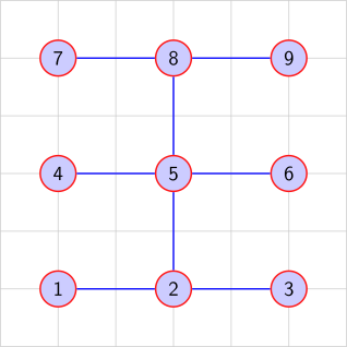
Figure 8: A Graph G” (N,T’) which is a
spanning tree of G (N, L)
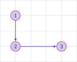
Figure 9: Arborescence of the Directed
Graph G (N, L)
3 Flows and Conservation Laws
When the links of a graph is used to denote flow of vehicles, goods, or pedestrain, then the
graph is referred as a network or transportation network
Flow then denotes quantity per unity time, the rate at which flow takes place (vehicles per
hour, pedestian per hour, etc.)
Fundamental to any network dealing with flows (like electrical, or water or transportation
network) is the fact that flows are not lost in the network.
Kirchhoff’s law state the same concept, but note that we are concerned with the steady state
macroscopic conditions and not valid under microscopic and stocastic conditions.
3.1 Link Flows and Kirchhoff’s Law
Three kind of nodes exist in transporation network:
Intermediate node: sum of all flows entering the node equals the sum of all flows leaving
the node
Production Centroid or source: the sum of all flows leaving the node equals the flow
produced at that node
Attraction Centroid: or sink: the sum of all flows entering the node equals the flows
attracted to that node
Following notations may be stated first:
\(f_{ij}\) is the link flow on the directed link (\(i\),\(j\))
\(a_i\) is the flow produced at the centroid (\(i\))
\(b_i\) is the flow attracted to the centroid (\(i\))
All flows are assumed to be non-negative (\(f_{ij},~a_i,~b_i\ge ~0\))
\(A(i)\) is the set of nodes after node \(i\), defined as: \begin {equation} A(i)=\{j|j\in N,~(i,j)\in L\} \end {equation}
\(B(i)\) is the set of nodes before node \(i\), defined as: \begin {equation} B(i)=\{j|j\in N,~(j,i)\in L\} \end {equation}
Now, the Kirchhoff’s flow conservation law for a directed transportion network [\(N;L\)] can be written as:
The last equation ensures some solution to the problem. Since, the no of links are normally more than
the number of node in typical transportation networks, the number of unknown exceeds the number of
equations and hence there will be mutiple solutions to this problem.
3.1.1 Numerical Illustration
Verify Kirchhoff’s law for the network given in figure 10 for node 2 and 3.
Figure 10: Network illustrating flow conservation
SolutionNode 2: For the node \(i\)=2, \(A(i=2)={3,~4}\) and \(B(i=2)={1,3}\)
If \(i=1\) is the origin node and \(i=n\) is the destination node, the node 1 is desgnated as the production zone with \(g\)
where \(g\) is the flow produced and zero flow attracted. Similarly, the node \(n\) is designated as the attraction
zone with \(g\) where \(g\) is the flow attracted and zero flow is produced.
The conservation equation for such a network can be written as:
where, \(g\) denote the flow value, and \(f_{ij}\) is the flow on link \(i,j\).
Theorem
The net flow across any cut-set \((X,\bar {X})\) separating the origin and destination is equal to the flow
value.
3.2.1 Numerical Illustration
Verify the above theorem that the net flow across the cut-set \((X,\bar {X})\) separating the origin 1 and destination 4 is
equal to the flow value of 7 for the network given in figure 11.
Figure 11: Network illustrating flow value across cut-set
Solution
The cut set is defined by \(X=\{1,3\}\) and \(\bar {X}=\{2, 4\}\)
The cut-set \((X,\bar {X})=\{(1,2),(3,2),(2,3)\}\)
The cut-set \((\bar {X},X)=\{(2,4)\}\)
The net flow \(f(X,\bar {X})-f(\bar {X},X)=3+3+2-1=7\).
The conservation equation can be conveniently represented in a matrix form. The node-link incidence
matrix in an \(n\times l\) matrix \(\bf E\) where the rows corresponds to nodes (\(i\))and the column corresponds to links \((j,k)\) and
each cell denoted by \(\delta ^i_{jk}\) defined as: \begin {equation} \delta ^i_{jk} = \left \{ \begin {array}{lr} +1 & \mathrm {if}~ i=j,\\ -1 & \mathrm {if}~ i=k,\\ 0 & \mathrm {otherwise}\\ \end {array} \right . \end {equation} For example ...
and the resultant flow value vector \(\bf g\) is \begin {equation} {\bf Ef=g} \end {equation} where \(\bf f\) is the vector of link flows, \(\bf g\) is the O-D vector.
Link flow is superimposition of chain flow. Define:
\(f_i\) is the set of links (\(i=1,2\dots l\))
\(h_j\) is the set of chains (\(j=1,2\dots m\))
\(h_j\) is the chain flow.
The flow value \(g\) is then the sum of all chain flows, that is: \begin {equation} g=\sum _{j}h_j \end {equation} To get the link flow, a term \(a_{ij}\) is defined as: \begin {equation} a_{ij} = \left \{ \begin {array}{ll} 1 & \mathrm {if~link}~i~\mathrm {is on chain}~m_j,\\ 0 & \mathrm {otherwise}\\ \end {array} \right . \end {equation} And
now the link flow \(f_i\) is given as: \begin {equation} f_i=\sum _{j}a_{ij}~h_j \end {equation} Note that the link flow from chain flow is unique whereas the chain flow
from the link flow is not unique. The above things can be written in a matrix form by first defining a link
chain incident matrix \(A_{l\times m}\) with \(a_{ij}\) as it elements. T Then, the link flow vector \(\bf f\) is given as: \begin {equation} {\bf f}_{l\times 1}={\bf A}_{j\times m}~{\bf h}_{m\times 1} \end {equation} Now, the scalar
flow value \(g\) can be given as: \begin {equation} g={\bf e}^T~{\bf h} \end {equation} where \(\bf e\) is a column vecotor of size \(m\) and all elements equals to
1.
3.3.1 Numerical Illustration
For the network given in Figure 12, the chain flows are given below. Find the link flows and the flow
values.
no
Chains
Chain Flow
m1
(1,2) (2,3) (3,4)
1
m2
(1,2) (2,4)
2
m3
(1,3) (3,2) (2,4)
3
m4
(1,3) (3,4)
1
Figure 12: A Single OD Network
Solution
The link chain incident matrix \({\bf A}_{l\times m}\) can be written as:
The cost could be time, distance, delay, or disutility etc. The following notations and definitions are
normally used in transporation network analysis.
Link cost: \(c_{ij}(f_{ij})\) is the average cost or cost per unit flow. The unit link cost is function of the flow
on that link.
Total link cost: which is flow dependent can be defined as \(f_{ij}\times c_{ij}(f_{ij})\).
Route cost: on a chain or a path from origin to destination is the sum of all the link costs of the
links that define the route can be expressed as: \begin {equation} C_{(n_1, n_r)}=\sum _{i=1}^{r-1}c_{(n_i,n_{i+1})} \end {equation}
Route cost with turn penalties: is defined as: \begin {equation} C_{(n_1, n_r)}=\sum _{i=1}^{r-1}\left [c_{(n_i,n_{i+1})} + p_{((n_i,n_{i+1}),(n_{i+1},n_{i+2}))}\right ] \end {equation} where \(p_{((n_i,n_{i+1}),(n_{i+1},n_{i+2}))}\) is the penalty for turning from the link \((n_i,n_{i+1})\) to
\((n_{i+1},n_{i+2})\).
Network cost: \(\mathcal C\) is the sum of all the total link cost of all the links of the network, and is given as:
\begin {equation} {\mathcal C}=\sum _{(i,j)}f_{ij}\times c_{ij}(f_{ij}) \end {equation}
If a link is prohibited for movement, it can represented by putting \(c_{ij}=\infty \) and if a turn is prohibited, it can
be represented by \(p_{(.)}=\infty \)
4 Network Algorithms
4.1 Minimal spanning tree
In a connected weighted graph, all spanning trees have n-1 edges and will have minimum or maximum
sum of the weights. Tow algorithms are proposed: Prims algorithm and Kruskal’s algorithm.
‘
4.1.1 Prims algorithm
Prims algorithm grows a spanning tree from a given vertex of a connected weighted graph G, iteratively
adding the cheapest edge from a vertex already reached to a vertex not yet reached, finishing when all the
vertices of G have been reached. Break tie arbitrarily.
Input:
G(N,L) weighted and connected
Initilize:
T(G)=\(\Phi \)
Iteration:
add cheapest edge that
incorporate a new vertex
Figure 13: Prims Algorithm
4.1.2 Numerical Example
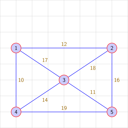
Find the minimum spanning tree of the network given in figure 14
Figure 14: Example network for minimum spanning tree problem 1
Solution
Start with node 1, N={1}, T={\(\Phi \)}
Node 1 can be connected by nodes 2, 3, and 4, having weights 12, 17, and 10
Minimum weight is 10, for node 4. So N={1,4}, T={(1,4)}
Node 1 can be connected by nodes 2 and 3, having weights 12 and 17
Node 4 can be connected by nodes 3 and 5, having weights 14 and 19
Minimum weight is 12, for node 2. So N={1,4,2}, T={(1,4),(1,2)}
Node 1 can be connected by node 3, having weight 17
Node 4 can be connected by nodes 3 and 5, having weights 14 and 19
Node 2 can be connected by nodes 3 and 5, having weights 18 and 16
Minimum weight is 14, for node 3. So N={1,4,2,3}, T={(1,4),(1,2),(3,4)}
Node 1 can be connected by no nodes without loop
Node 4 can be connected by node 5, having weight 19
Node 2 can be connected by node 5, having weight 16
Node 3 can be connected by node 5, having weight 11
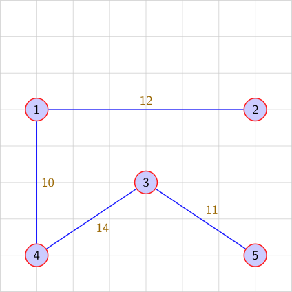
Minimum weight is 11, for node 3. So N={1,4,2,3}, T={(1,4),(1,2),(3,4),(3,5)} W=49.
Figure 15: Solution for the example network for minimum spanning tree problem 1
4.1.3 Kruskal’s algorithm
The main concept of this algorithm is to maintain an acyclic spanning sub-graph H, enlarging it by edges
with low weight to form a spanning tree. Consider edges in non-descending order of weight, breaking ties
arbitrarily.
Input:
G(N,L) weighted and connected
Initilize:
set T=\(\Phi \) a sub-graph of G
Iterate:
If the next cheapest edge joins
two components of T, then include
it, otherwise, discard it.
Terminate:
when T is connected
Figure 16: Kruskal Algorithm
Example
Find the minimum spanning tree of the network given in figure 14
Solution
Sort the links in the descending order of weights results in
This algorithm finds the shortest path for a graph from a starting node to every other node. The
algorithm is given in Figure 17 and each step is described below.
Input to the algorithm is a graph \(G(N,L) \) with nonnegative edge weights and a starting vertex \(u\). The
destination vertex \(v\) The weight of the edge \(xy\) is \(w(xy)\) and \(w(xy)=\infty \) if \(xy\) is not an edge.
Initilize step involves defining the solution set \(S\) with the starting vertex as the only element.
Further, a variable \(t\) associated with vertex \(u\) is defined and set its value to zero.
Iteration starts by selecting all possible edges defined by the starting node \(v\) from the set \(S\) and
the end node \(z\) not in the set \(S\). For each of the end node \(z\), the total cost up to that node is
computed by adding the total cost upto node \(v\) computed in previos iteration and the weight of
the edge \((xy)\), that is \(t(z)=t(v)+w(xy)\). Find the node which has minimum cost and add that node to the solution
set \(S\).
Termination of the algorithm happens when all the node becomes element of the solution set
\(S\) or the destination node is reached.
1
Input
\(G(N,L)\), \(w(xy)\ge 0\), \(u\)
2
Initilize
\(S=\{u\}\)
3
\(t(u)=0\)
4
Iterate
select \(v\in S\) and \(z\notin S\)
5
such that \(t^{*}(z)\)=Min \(t(z)\)
6
where \(t(z)=t(v)+w(vz)\)
7
set \({S}^* = {S} \cup z\)
8
Terminate
till \(S=V\{G\}\)
Figure 17: Dijkstra’s Shortest Path Algorithm
4.2.1 Numerical Example
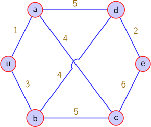
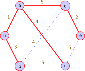
Find the minimum shortest path of the graph given in figure 18 from the node u.
Figure 18: Example network for shortest path problem 1
Solution
Table 1: Solution to the shortest path algorithm
\(\{S\}\)
\(v\)
\(vz\)
\(t(z)\)
\(t^*(z)\)
\(z^*\)
\(\{S^*\}\)
u
u
ua
0+1=1
1
a
ua
ub
0+3=3
ua
u
ub
0+3=3
3
b
uab
a
ad
1+5=6
ac
1+4=4
uab
a
ad
1+5=6
ac
1+4=5
5
c
uabc
b
bd
3+4=7
bc
3+5=8
uabc
a
ad
1+5=6
6
d
uabcd
b
bd
3+4=7
c
ce
5+6=11
uabcd
d
de
6+2=8
8
e
uabcde
c
de
5+6=11
Note: \(t(z)=t(v)+w(vz)\), \(t^*(z)=min~t(z)\)
Figure 19: Example network for shortest path problem 1
4.2.2 Numerical Example 2
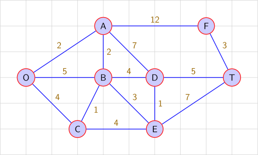
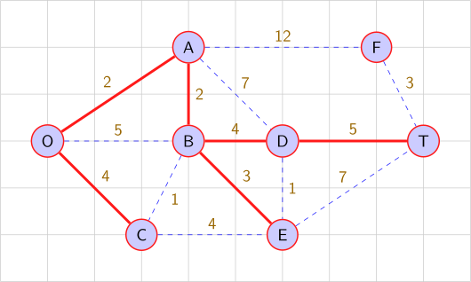
Find the minimum shortest path of the graph given in figure 20 from the node O to the destination node
T.
Figure 20: Example network for shortest path problem 1
Figure 21: Solution to the example network for shortest path problem 1
5 Network Optimization
5.1 Maximum Flow Problem
5.2 Minimum Cost Flow Problem
5.3 Transportation Problem
5.4 Assignment Problem
5.5 Traveling Salesman Problem
6 Travelling salesman problem (TSP)
6.1 Introduction
Travelling salesman problem (TSP) consists of finding the shortest rout e in complete weighted graph G
with n nodes and n(n-1) edges, so that the start node and the end node are identical and all other nodes
in this tour are visited exactly once.
6.2 Formulation
Let \(\bf C\) be the matrix of shortest distances (dimension \(nxn\)), where \(n\) is the number of nodes of graph \(G(NL)\). The
elements of matrix \(\bf C\) represents the shortest distances between all pairs of nodes \((i,j), i, j =1, 2, \dots , n\). The travelling salesman
problem can be formulated in the category programming binary, where variables are equal to 0
or 1, depending on the fact whether the route from node \(i\) to node \(j\) is realized (\(x_{ij}=1\)) or not (\(x_{ij}=0\)).
Then, the mathematical formulation of TSP is as follows (the idea of this formulation is to
assign the numbers \(1\) through \(n\) to the nodes with the extra variables \(u_i\), so that this numbering
corresponds to the order of the nodes in the tour. It is obvious that this excludes sub-tours,
as a sub-tour excluding the node \(1\) cannot have a feasible assignment of the corresponding \(u_i\)
variables):
\begin {gather} \mathrm {Min~}=\sum _{i=1}^{n}\sum _{j=1}^{n} c_{ij}~x_{ij}\\ {\mathrm {subjected~to}}\\ \sum _{i=1}^{n} x_{ij}=1,~~~j=1,2,\dots ,n;~~i \neq j\\ \sum _{j=1}^{n} x_{ij}=1,~~~i=1,2,\dots ,n;~~i\neq j\\ u_i-u_j+n~x_{ij}\leq n-1, i,j=2,3,\dots ,n;~~i\neq j\label {qeTSPd}\\ x_{ij}\in \{0,1\}1,~~~i=1,2,\dots ,n;~~i\neq j \end {gather} The constraint ?? ensures there is no sub-trours.
Exercises
Not Available
References
Frederick S Hillier and Gerald J Lieberman. Introduction to Operations Research. Tata
McGraw-Hill Publishers, New Delhi, 2001.
Renfrey B Potts and Robert M Oliver. Flows in transportation networks. Academic Press,
New York, 1972.
Douglas B West. Introduction to graph theory. Pearson education Asia, New Delhi, India,
2001.
Acknowledgments
I wish to thank several of my students and staff of NPTEL for their contribution in this lecture. I
also appreciate your constructive feedback which may be sent to tvm@civil.iitb.ac.in. Prof.
Tom V. Mathew, Department of Civil engineering, Indian Instiute of Technology Bombay,
India.