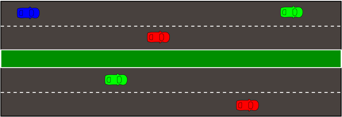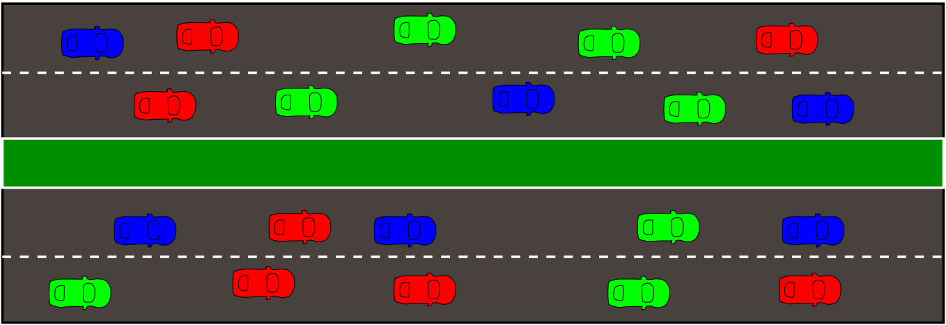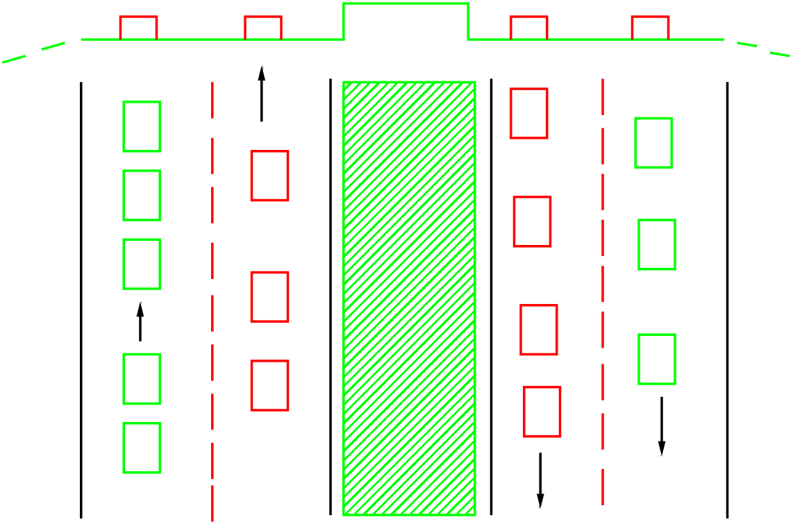
Figure 1: Divided multilane highway in a rural/suburban environment
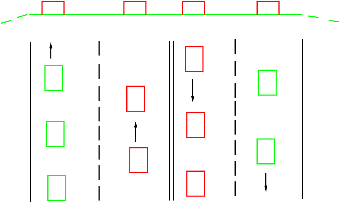
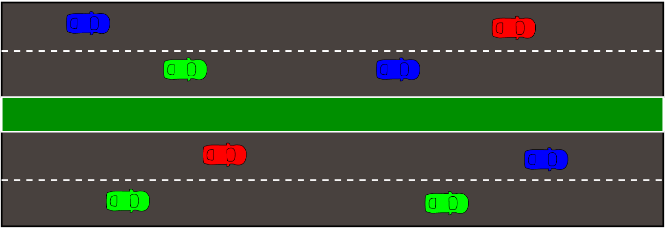
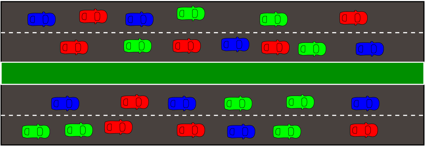
Figure 2: Undivided multilane highway in a rural/suburban environment
Increasing traffic flow has forced engineers to increase the number of lanes of highways in order to provide good manoeuvring facilities to the users. The main objectives of this lecture is to analyze LOS which is very important factor for a traffic engineer because it describes the traffic operational conditions within a traffic stream. Also we are going to study the characteristics and capacity for multilane highways. Free-flow speed is an important parameter that is being used extensively for capacity and level-of- service analysis of various types of highway facilities.
A highway is a public road especially a major road connecting two or more destinations. A highway with at least two lanes for the exclusive use of traffic in each direction, with no control or partial control of access, but that may have periodic interruptions to flow at signalized intersections not closer than 3.0 km is called as multilane highway. They are typically located in suburban areas leading to central cities or along high-volume rural corridors that connect two cities or important activity centers that generate a considerable number of daily trips.
There are various ways of classification of highways; we will see classification of highways according to number of lanes.
Multilane highways generally have posted speed limits between 60 km/h and 90 km/h. They usually have four or six lanes, often with physical medians or two-way right turn lanes (TWRTL), although they may also be undivided. The traffic volumes generally varies from 15,000 - 40,000 vehicles per day. It may also go up to 100,000 vehicles per day with grade separations and no cross-median access. Traffic signals at major intersections are possible for multilane highways which facilitate partial control of access. Typical illustrations of multilane highway configurations are provided in Fig. 1 and 2
An important operation characteristic of any transport facility including the multi lane highways is the concept of capacity. Capacity may be defined as the maximum sustainable flow rate at which vehicles or persons reasonably can be expected to traverse a point or uniform segment of a lane or roadway during a specified time period under given roadway, traffic, environmental, and control conditions; usually expressed as vehicles per hour, passenger cars per hour, or persons per hour. There are two types of capacity, possible capacity and practical capacity. Possible capacity is defined as the maximum number of vehicles that can pass a point in one hour under prevailing roadway and traffic condition. Practical capacity on the other hand is the maximum number that can pass the point without unreasonable delay restriction to the average driver’s freedom to pass other vehicles. Procedure for computing practical capacity for the uninterrupted flow condition is as follows:
| Types of facility | Free flow | Capacity |
| speed(kmph) | (pcphpl) | |
| Multilane | 100 | 2200 |
| 90 | 2100 | |
| 80 | 2000 | |
| 70 | 1900 | |
Level of service (LOS) is a qualitative term describing the operational performance of any transportation facility. The qualitative performance measure can be defined using various quantitative terms like:
Basically any two of the following three performance characteristics can describe the LOS for a multilane highway. Each of these measures can indicate how well the highway accommodates the traffic demand since speed does not vary over a wide range of flows, it is not a good indicator of service quality. Density which is a measure of proximity of other vehicles in the traffic stream and is directly perceived by drivers and does not vary with all flow levels and therefore density is the most important performance measure for estimating LOS. Based on the quantitative parameter, the LOS of a facility can be divided into six qualitative categories, designated as LOS A,B,C,D,E,F The definition of each level of service, is given below:
Travel conditions are completely free flow. The only constraint on the operation of vehicles lies in the geometric features of the roadway and individual driver preferences. Lane changing, merging and diverging manoeuvre within the traffic stream is good, and minor disruptions to traffic are easily absorbed without an effect on travel speed. Average spacing between vehicles is a minimum of 150 m or 24 car lengths. Fig. 3 shows LOS A.
Travel conditions are at free flow. The presence of other vehicles is noticed but it is not a constraint on the operation of vehicles as are the geometric features of the roadway and individual driver preferences. Minor disruptions are easily absorbed, although localized reduction in LOS are noted. Average spacing between vehicles is a minimum of 150 m or 24 car lengths. Fig. 4 below shows LOS B.
Traffic density begins to influence operations. The ability to manoeuvre within the traffic stream is affected by other vehicles. Travel speeds show some reduction when free-flow speeds exceed 80 km/h. Minor disruptions may be expected to cause serious local deterioration in service, and queues may begin to form. Average spacing between vehicles is a minimum of 150 m or 24 car length. Fig. 5 shows LOS C.
The ability to manoeuvre is severely restricted due to congestion. Travel speeds are reduced as volumes increase. Minor disruptions maybe expected to cause serious local deterioration in service, and queues may begin to form. Average spacing between vehicles is a minimum of 150 m or 24 car length. Fig. 6 shows LOS D.
Operations are unstable at or near capacity. Densities vary, depending on the free-flow speed. Vehicles operate at the minimum spacing for which uniform flow can be maintained. Disruptions cannot be easily dissipated and usually result in the formation of queues and the deterioration of service to LOS F. For the majority of multilane highways with free-flow speed between 70 and 100km/h, passenger-car mean speeds at capacity range from 68 to 88 km/h but are highly variable and unpredictable. Average spacing between vehicles is a minimum of 150 m or 24 car length. Fig. 7 shows LOS E.
A forced breakdown of flow occurs at the point where the numbers of vehicles that arrive at a point exceed the number of vehicles discharged or when forecast demand exceeds capacity. Queues form at the breakdown point, while at sections downstream they may appear to be at capacity. Operations are highly unstable, with vehicles experiencing brief periods of movement followed by stoppages. Travel speeds within queues are generally less than 48 km/h. Note that the term LOS F may be used to characterize both the point of the breakdown and the operating condition within the queue. Fig. 8 shows LOS F.
The determination of level of service for a multilane highway involves three steps:
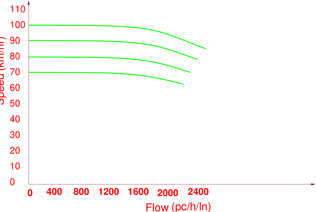
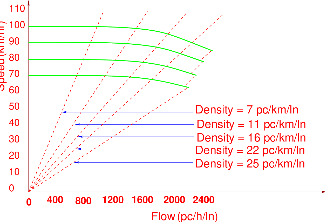
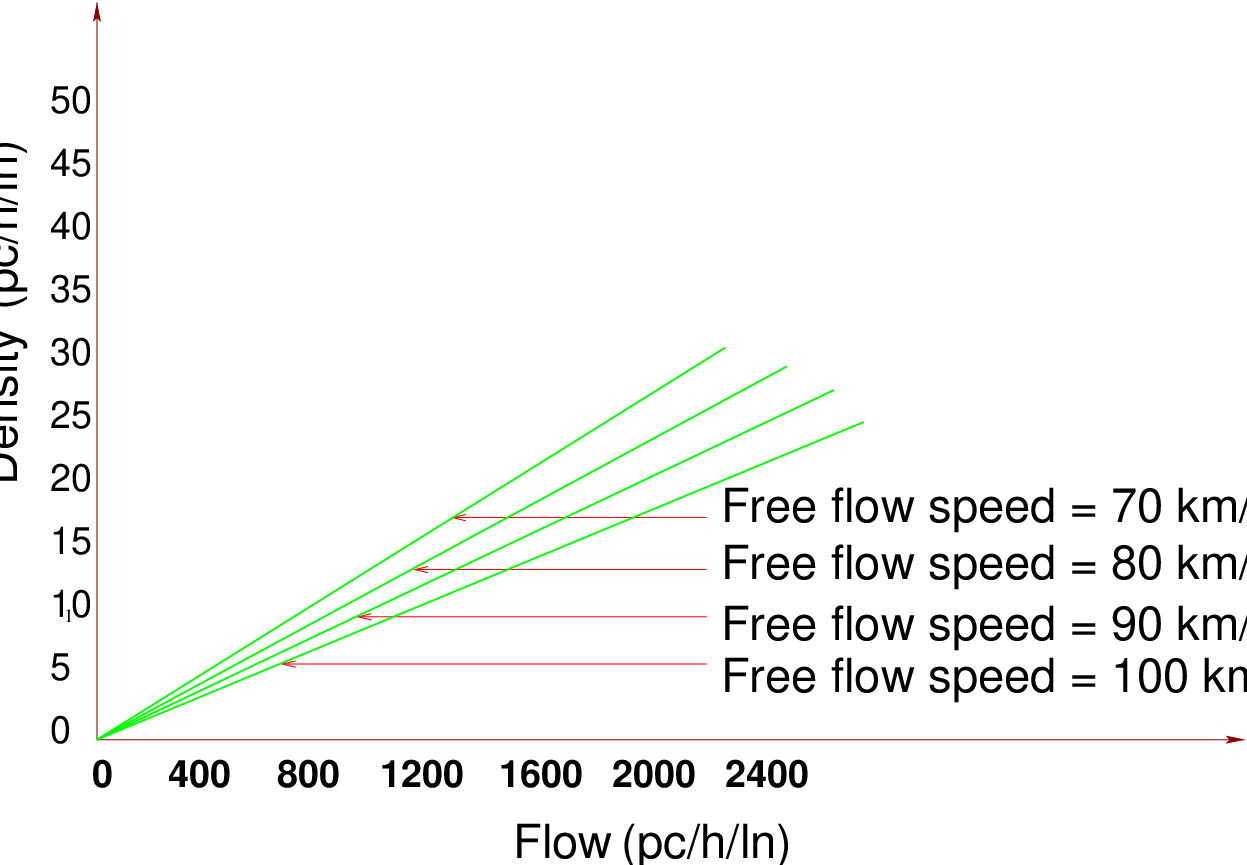
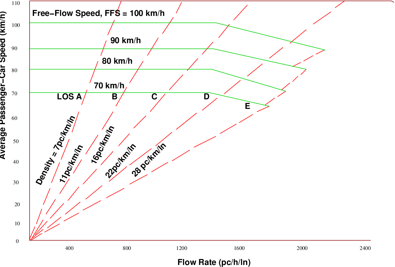
Free-flow speed is the theoretical speed of traffic density, when density approaches zero. It is the speed at which drivers feel comfortable travelling under the physical, environmental and traffic conditions existing on an uncongested section of multilane highway. In practice, free-flow speed is determined by performing travel-time studies during periods of low-to-moderate flow conditions. The upper limit for low to moderate flow conditions is considered 1400 passenger cars per hour per lane(pc/h/ln) for the analyses. Speed-flow and density flow relationships are shown in Fig. 9 and Fig. 10. These relationships hold for a typical uninterrupted-flow segment on a multilane highway under either base or no base conditions in which free-flow speed is known. Fig. 9 indicates that the speed of traffic volume up to a flow rate of 1400 pc/h/ln. It also shows that the capacity of a multilane highway under base conditions is 2200 pc/h/ln for highways with a 90 km/h free-flow speed. At flow rates between 1400 and 2200 pc/h/ln, the speed on a multilane highway drops; for example, by 8 km/h for a highways with a free-flow speed of 90 km/h. Fig. 10 shows that density varies continuously throughout the full range of flow rates. The capacity value of 2200 pc/h/ln is representative of the maximum 15-min flow rate that can be accommodated under base conditions for highways with 90 km/h free-flow speed.
From various studies of the flow characteristics, base conditions for multilane highways are defined as follows:
The average of all passenger-car speeds measured in the field under low volume conditions can be used directly as the free-flow speed if such measurements were taken at flow rates at or below 1400 pc/h/ln. No adjustments are necessary as this speed reflects the net effect of all conditions at the site that influence speed, including lane width, lateral clearance, type of median, access points, posted speed limits, and horizontal and vertical alignment. Free-flow speed also can be estimated from 85th-percentile speed or posted speed limits, research suggests that free-flow speed under base conditions is 11 km/h higher than the speed limit for 65 km/h to 70 km/h speed limits and 8 km/h higher for 80 km/h to 90 km/h speed limits. Fig. 12 shows speed-flow curves with LOS criteria for multilane highways, here LOS is easily determined for any value of speed simply by plotting the point which is a intersection of flow and corresponding speed. Note that density is the primary determinant of LOS. LOS F is characterized by highly unstable and variable traffic flow. Prediction of accurate flow rate, density, and speed at LOS F is difficult.
| Free-Flow | Criteria | (LOS) | (LOS) | (LOS) | (LOS) | (LOS) |
| Speed | A | B | C | D | E | |
| 100 km/h | Max. density | 7 | 11 | 16 | 22 | 25 |
| (pc/km/ln) | ||||||
| Average speed | 100 | 100 | 98.4 | 91.5 | 88 | |
| (kmph) | ||||||
| Max. volume | 0.32 | 0.50 | 0.72 | 0.92 | 1.00 | |
| capacity ratio | ||||||
| Max. service | 700 | 1100 | 1575 | 2015 | 2200 | |
| flow rate | ||||||
| (pc/h/ln) | ||||||
When field data are not available, the free-flow speed can be estimated indirectly as follows:
 | (1) |
where, FFS is the estimated FFS (km/h), BFFS= base FFS (km/h), fLW= adjustment for lane width, from Table 3 (km/h), fLC= adjustment for lateral clearance, from Table 4 (km/h), fM= adjustment for median type, from Table 5 (km/h), and fA= adjustment for access points, from Table 6 (km/h). FFS on multilane highways under base conditions is approximately 11 km/h higher than the speed limit for 65 and 70 km/h speed limits, and it is 8 km/h higher for 80 and 90 km/h speed limits. BFFS is approximately equal to 62.4 km/h ( i.e decrease in 1.6 km/h) when the 85 th percentile speed is 64 km/h, and it is 91.2 km/h ( i.e decrease in 4.8 km/h) when the 85 th percentile speed is 96 km/h and the in between speed values is found out by interpolation.
| Lane Width (m) | Reduction in FFS(km/h) | |||||
| 3.6 | 0.0 | |||||
| 3.5 | 1.0 | |||||
| 3.4 | 2.1 | |||||
| 3.3 | 3.1 | |||||
| 3.2 | 5.6 | |||||
| 3.1 | 8.1 | |||||
| 3.0 | 10.6 | |||||
According to Table 3, the adjustment in km/h increase as the lane width decreases from a base lane width of 3.6 m. No data exist for lane widths less than 3.0m.
The adjustment for lateral clearance (TLC) is given as:
 | (2) |
where, TLC = Total lateral clearance (m), LCL = Lateral clearance (m), from the right edge of the travel lanes to roadside obstructions (if greater than 1.8 m, use 1.8 m), and LCR= Lateral clearance (m), from the left edge of the travel lanes to obstructions in the roadway median (if the lateral clearance is greater than 1.8 m, use 1.8 m). Once the total lateral clearance is computed, the adjustment factor is obtained from Table 4.
| Four-Lane Highways | Six-Lane Highways
| ||
| Total Lateral | Reduction in FFS | Total Lateral | Reduction in FFS |
| Clearance a (m) | (km/h) | Clearance a (m) | (km/h) |
| 3.6 | 0.0 | 3.6 | 0.0 |
| 3.0 | 0.6 | 3.0 | 0.6 |
| 2.4 | 1.5 | 2.4 | 1.5 |
| 1.8 | 2.1 | 1.8 | 2.1 |
| 1.2 | 3.0 | 1.2 | 2.7 |
| 0.6 | 5.8 | 0.6 | 4.5 |
| 0.0 | 8.7 | 0.0 | 6.3 |
| Median Type | Reduction in FFS (km/h) |
| Undivided highways | 2.6 |
| Divided highways | 0.0 |
For undivided highways, there is no adjustment for the right-side lateral clearance as this is already accounted for in the median type. Therefore, in order to use Table 5 for undivided highways, the lateral clearance on the left edge is always 1.8 m, as it for roadways with TWRTLs.
| Access Points/Kilometer | Reduction in FFS (km/h) |
| 0 | 0.0 |
| 6 | 4.0 |
| 12 | 8.0 |
| 18 | 12.0 |
| ≥ 24 | 16.0 |
The access-point density, which is use in Table 6, for a divided roadway is found by dividing the total number of access points (intersections and driveways) on the right side of the roadway in the direction of travel being studied by the length of the segment in kilometers. The adjustment factor for access-point density is given in Table 6. Thus the free flow speed can be computed using equation 1 and applying all the adjustment factors.
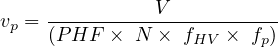
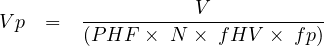
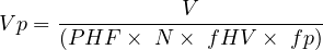
The next step in the determination of the LOS is the computation of the peak hour factor. The fifteen minute passenger-car equivalent flow rate (pc/h/ln), is determined by using following formula:
 | (3) |
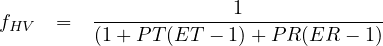
where, vp is the 15-min passenger-car equivalent flow rate (pc/h/ln), V is the hourly volume (veh/h), PHF is the peak-hour factor, N is the number of lanes, fHV is the heavy-vehicle adjustment factor, and fp is the driver population factor. PHF represents the variation in traffic flow within an hour. Observations of traffic flow consistently indicate that the flow rates found in the peak 15-min period within an hour are not sustained throughout the entire hour. The PHFs for multilane highways have been observed to be in the range of 0.75 to 0.95. Lower values are typical of rural or off-peak conditions, whereas higher factors are typical of urban and suburban peak-hour conditions. Where local data are not available, 0.88 is a reasonable estimate of the PHF for rural multilane highways and 0.92 for suburban facilities. Besides that, the presence of heavy vehicles in the traffic stream decreases the FFS because base conditions allow a traffic stream of passenger cars only. Therefore, traffic volumes must be adjusted to reflect an equivalent flow rate expressed in passenger cars per hour per lane (pc/h/ln). This is accomplished by applying the heavy-vehicle factor (fHV ). Once values for ET and ER have been determined, the adjustment factors for heavy vehicles are applied as follows:
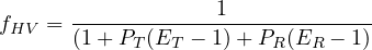 | (4) |
where, ET and ER are the equivalents for trucks and buses and for recreational vehicles (RVs), respectively, PT and PR are the proportion of trucks and buses, and RVs, respectively, in the traffic stream (expressed as a decimal fraction), fHV is the adjustment factor for heavy vehicles. Adjustment for the presence of heavy vehicles in traffic stream applies for three types of vehicles: trucks, buses and recreational vehicles (RVs). Trucks cover a wide range of vehicles, from lightly loaded vans and panel trucks to the most heavily loaded coal, timber, and gravel haulers. An individual truck’s operational characteristics vary based on the weight of its load and its engine performance. RVs also include a broad range: campers, self-propelled and towed; motor homes; and passenger cars or small trucks towing a variety of recreational equipment, such as boats, snowmobiles, and motorcycle trailers. There is no evidence to indicate any distinct differences between buses and trucks on multilane highways, and thus the total population is combined.
| Factor | Type of Terrain
| ||
| Level | Rolling | Mountainous | |
| ET (Trucks and Buses) | 1.5 | 2.5 | 4.5 |
| ER (RVs) | 1.2 | 2.0 | 4.0 |
The level of service on a multilane highway can be determined directly from Fig. 12 or Table-2 based on the free-flow speed (FFS) and the service flow rate (vp) in pc/h/ln. The procedure as follows:
In general, the minimum length of study section should be 760 m, and the limits should be no closer than 0.4 km from a signalized intersection.
 | (5) |
where, D is the density (pc/km/ln), vp is the flow rate (pc/h/ln), and S is the average passenger-car travel speed (km/h). The level of service can also be determined by comparing the computed density with the density ranges shown in table given by HCM. To use the procedures for a design, a forecast of future traffic volumes has to be made and the general geometric and traffic control conditions, such as speed limits, must be estimated. With these data and a threshold level of service, an estimate of the number of lanes required for each direction of travel can be determined.
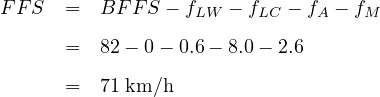
A segment of undivided four-lane highway on level terrain has field-measured FFS 74.0-km/h, lane width 3.4-m, peak-hour volume 1,900-veh/h, 13 percent trucks and buses, 2 percent RVs, and 0.90 PHF. What is the peak-hour LOS, speed, and density for the level terrain portion of the highway?
Solution The solution steps are given below:
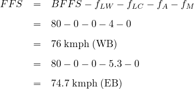
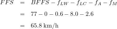
A segment of an east-west five-lane highway with two travel lanes in each direction separated by a two-way left-turn lane (TWLTL) on a level terrain has- 83.0-km/h 85th-percentile speed ,3.6-m lane width, 1,500-veh/h peak-hour volume, 6 % trucks and buses, 8 access points/km (WB), 6 access points/km (EB), 0.90 PHF, 3.6-m and greater lateral clearance for westbound and eastbound. What is the LOS of the highway on level terrain during the peak hour?
Solution The solution steps are enumerate below:
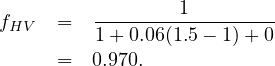
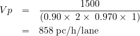
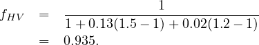
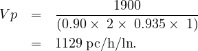
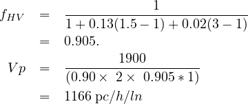
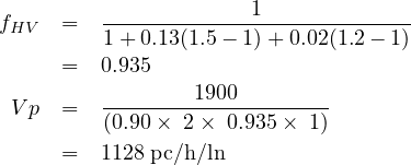
A 10 km long 4 lane undivided multilane highway in a suburban area has a segment 1 km long with a 3% upgrade and a segment 1 km long with a 3% downgrade. The section has a volume of 1900 vehicles/hr in each direction with 13% trucks and buses and 2% recreational vehicles. The 85 th percentile speed of passenger car is 80 km/hr on upgrade and 86km/hr on downgrade. There are total of 12 access points on both sides of the roadway. The lane width is 3.6 m, PHF is 0.90 and having a 3m lateral clearance. Determine the LOS of the highway section (upgrade and downgrade) during the peak hour? From HCM, For a 3% upgrade and 1 km length( ET=1.5 , ER=3) For a 3% downgrade and 1 km length( ET=1.5 , ER=1.2 )
For upgrade: Flow rate is calculated from the equation

For downgrade:
This chapter helps to determine the level of service and capacity for a given road segment. In the first part we studied highways in general there classification and characteristics which gives the overall idea of multilane highways. Then we studied determination of capacity for multilane highway which is again a very important parameter used to determine the level of service, then we studied the concept of level of service and procedure to determine level of service. Also by using its applications, number of lanes required (N), and flow rate achievable (vp), Performance measures related to density (D) and speed (S) can also be determined.
I wish to thank several of my students and staff of NPTEL for their contribution in this lecture. I wish to thank specially my student Mr. Digviyay S. Pawar for his assistance in developing the lecture note, and my staff Mr. Rayan and Ms. Reeba in typesetting the materials. I also appreciate your constructive feedback which may be sent to tvm@civil.iitb.ac.in
Prof. Tom V. Mathew
Department of Civil Engineering
Indian Institute of Technology Bombay, India
_________________________________________________________________________
Wednesday 27 September 2023 10:44:18 PM IST