Contents

1 Introduction

Transport problems are very critical one to be solved frequently, sequentially and economically for all sectors of one nation. Even though these solutions are mandatory, they are continuous and expensive so needs to be planned systematically. These all requirements will lead us to Transportation System Planning. Transportation System Planning is a tool that attempts to provide feasible and systematic method for solving transport problems of the society. Transportation system planning starts from the problem of the society which is the difference of users desire to the existing condition of the system. Afterwards following its stages it will attempt to meet its goals and objectives. While in the process so many analyses are required to be done from them the one is done to know the performance of the existing system. This can be expressed as either individual component performance or the whole system performance. Doing this is dependent on the type of transportation system. Among them multi modal multi facility system is the one which requires aggregate performance measurement for all components which constitutes. According to our study area we can choose from the two methods of performance measurement alternatives which are Corridor analysis and Area wide analysis.

2 Terminologies

The terminologies used in the corridor analysis is provided below.

2.1 Corridor system

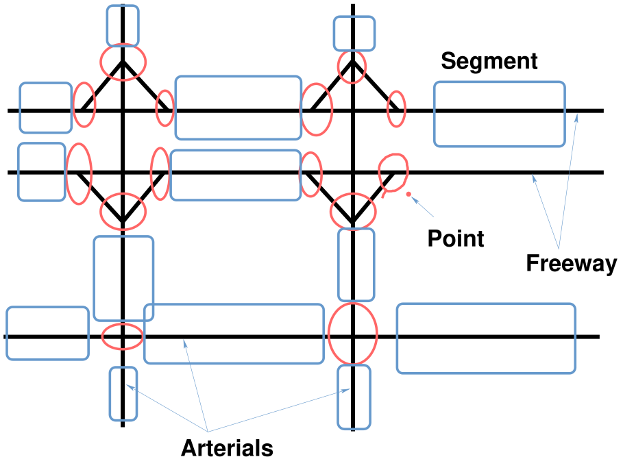
1. Corridor: A corridor is a set of essentially parallel and competing facilities and modes with cross-connectors that serve trips between two designated points. A corridor may contain several subsystems of facilities freeway, rural highway, urban street, transit, pedestrian, and bicycle Figure. 1.

   

2. Segment: Segments are stretches of a facility in which the traffic demand and capacity conditions are relatively constant.
3. Point: Points are locations at the beginning and end of each segment, at which traffic enters, leaves, or crosses the facility.
4. Facility: is a structure built or road design modification to increase the efficiency of the two main road way services (accessibility and Mobility).

2.2 Highway sub systems

1. Freeway: A freeway is defined as a divided highway with full control of access and having two uninterrupted flow or more lanes for the exclusive use of traffic in each direction. All the access is through a ramp a separate entrance or exit way to or from the Freeway.
2. Rural highway: A road with only one lane in each direction and traffic signals spaced no closer than 3.0 km. mostly recognized by its low flow condition.
3. Urban Street: With traffic signals spaced no farther than 3.0 km apart. Since in Urban areas most activities are fond of Transportation, are characterized by its high flow condition and high traffic movements due the complex interaction between vehicles accidents are also high in urban areas. To avoid this and other conflicts Traffic control is required especially in urban areas.

2.3 Transit

Transits are a means of transporting massive either passenger or freight on a separated route. These modes of transportations are a key to every city especially in urban areas. The most common types of Transits include:

1. Bus transit is a term applied to a variety of public transportation systems using buses to provide faster, more efficient service than an ordinary bus line. Often this is achieved by making improvements to existing infrastructure, vehicles and scheduling. Bus rapid transit also called Bus way and/or Quality bus.
2. Street car is a means of public transport which requires their own rail to flow through the system these rails can be built embedded in roadways. Streetcar (also called Tram) is a passenger rail vehicle which runs on tracks along public urban streets and also sometimes on separate rights of way.
3. Rail transit is a form of urban rail public transportation that generally has a lower capacity and lower speed than heavy rail and metro systems, but higher capacity and higher speed than traditional street-running tram systems.

3 Segment capacity

Capacity is the maximum hourly flow rate, at which persons or vehicles reasonably can be expected to traverse a point or a uniform section, of a lane or roadway during a given time period, under prevailing roadway, traffic and control conditions. But sometimes the demand may exceed the capacity during peak hours, which will bring queue delay. Thus demand adjustment is required and is done as follows. Adjusting for excess demand from the capacity is necessary only if working with forecasted or estimated demands rather than counted traffic. If the demand exceeds the capacity at any point in time or space, then the excess demand must be stored on the segment and carried over to the following hour. The downstream demands are reduced by the amount of excess demand stored on the segment. The algorithm starts with the entry gate segments on the periphery of the corridor and works inward until all segment demands have been checked against their capacity.

3.1 Demand adjustment algorithm

The following steps are used to adjust demand when excess demand occurs in a time period.

1. Step 1. Select the entry gate segment with the highest priority and the highest v/c ratio.
2. Step 2. Select the first time period.
3. Step 3. If demand \(\leq \) capacity or the initial queue = 0, go to Step 7.
4. Step 4. If demand \(>\) capacity or queue \(>\) 0, then calculate new queue by using eqn. 1. \begin {equation} {\mathrm {queue}}_i={\mathrm {queue}}_{i-1}+{\mathrm {demand}}-{\mathrm {capacity}} \label {qeCorQueue} \end {equation} where, \(i\) is the current analysis period, \(i-1\) is the previous analysis period, \(queue_{i-1}\) is the queue remaining from the preceding analysis period.
5. Step 5. Reduce downstream segment demand by the amount that the demand exceeds the capacity. Propagate this reduction to all connecting downstream segments in proportion to the ratio of each downstream segment demand to all segments exiting from the subject segment. Continue the process downstream until the reduction is less than 5 percent of capacity.
6. Step 6. Add the excess demand - the amount by which the demand exceeds the capacity - to the next time period demand for the subject segment.
7. Step 7. Apply the increment to the next time period. Repeat Steps 3 through 6 until the processes for all the time periods are finished.
8. Step 8. Go to next gate tree with unanalyzed segments in current rank. Repeat Steps 2 through 7 until all segments of current rank have been analyzed.
9. Step 9. Apply the increment to current Rank (the new one). Go to the segment with the highest v/c ratio among those of the new rank. Repeat Steps 2 through 8 until all segments are analyzed.

3.2 Free flow Travel time

The segment free-flow traversal times are obtained by dividing the length of the segment by the estimated free-flow speed (FFS), as shown in equation 2 \begin {equation} R_f = \frac {L}{S_f} \label {qeCorTravelTime} \end {equation} where, \(R_f\) is the Segment free-flow travel time for given Direction of Segment and Time Period, (hr), \(L\) is the length of segment (km), and \(S_f\) is the Segment free-flow speed computed (km/hr). The FFS is computed according to the Part III methods using the adjusted demands determined in the previous step. The computation is repeated for each direction of each segment for each time sub-periods.

3.3 Queue delay

The queuing delay only the amount due to demand exceeding capacity is computed for all segments. The queuing delay is computed for each direction of each segment and time period only when demand is greater than Capacity by eqn. 3. \begin {equation} D_i = \frac {T}{2} \times D_{i-1} + [V-c] \times \frac {T^2}{2} \label {qeCorDelay} \end {equation} where, \(D_i\) is the total delay due to excess demand (veh-hr) for direction, segment, and time period; \(T\) is the duration of time sub-period (hr); \(D_{i-1}\) is the queue left over at end of previous time period (veh); \(V\) is the demand rate for current time period (veh/hr); and \(c\) is the capacity of segment in subject direction (veh/hr). These the above steps are repeated for any additional time periods to be analyzed. For example, if the peak period lasts for 4 hours, it might be divided into four 1hr periods (or 16 quarter hr periods), with each time period analyzed in sequence. The first and the last analysis periods must be uncongested for all delay to be included in the performance measures. Once all time periods have been analyzed, the performance measures are computed.

4 Determining performance measures

This step describes how to compute performance measures of congestion intensity, duration, extent, variability, and accessibility for the corridor.

4.1 Intensity

The possible performance measures for the intensity of congestion on the highway subsystems (freeway, two-lane highway, and arterial) in the corridor are computed from one or more of the following: person-hours of travel, person-hours of delay, mean trip speed, and mean trip delay. If average vehicle occupancy (AVO) data are not available, then the performance measures are computed in terms of vehicle-hours rather than person-hours.

1. The eqn. 4 given below is used to determine PHT. \begin {equation} PHT = AVO \times \Sigma _{d,l,h}[V \times R + DQ] \label {qeCorPHT} \end {equation} where, \(PHT\) is the person-hours of travel in corridor, \(AVO\) is the average vehicle occupancy, \(V \) is the vehicle demand in Direction on Link during Time Period (veh), \(R\) is the segment traversal time (h/km), and \(DQ\) is the queuing delay (veh-h).
2. The mean trip time is computed by dividing the total person hours of travel by the number of person trips. \begin {equation} t=60 \times PHT/P \label {qeCorMeanTripTime} \end {equation} where, \(t\) is the mean trip time (min/person), \(PHT\) is the person-hours of travel, and \(P\) is the total number of person trips.
3. The mean trip speed is computed by dividing the total number of person-kilometers by the total person-hours of travel as in eqn. 6 below: \begin {equation} S = \frac {PkmT}{PHT} =AVO \times \frac {\Sigma _{d,l,h}[V \times L]}{PHT} \label {qeCorTripSpeed} \end {equation} where, \(S\) is the mean corridor trip speed (km/h), \(PkmT\) is the person-kilometers of travel, PHT is the person-hours of travel, \(AVO\) is the average vehicle occupancy, \(V\) is the vehicle demand in the given Direction on a Segment and Period (veh), and \(L\) is the length of segment (km).
4. The mean trip delay is computed by subtracting the PHT under free-flow conditions from the PHT under congested conditions and dividing the result by the number of person-trips. The person-hours of travel under free-flow conditions is computed like PHT for congested conditions, but using free-flow traversal times and zero queuing delay. It can be determined using eqn. 7 given below: \begin {equation} d = 3600 \times \frac {(PHT-PHT_f)}{P} \label {qeCorMeanTripDelay} \end {equation} where, \(d\) is the mean trip delay (s/person), \(PHT\) is the person-hours of travel, \(PHT_f\) is the person-hours of travel under free-flow conditions, and \(P\) is the total number of person trips.

4.2 Duration

Performance measurements of duration can be computed from the number of hours of congestion observed on any segment. The duration of congestion is the sum of the length of each analysis sub-periods for which the demand exceeds capacity. The duration of congestion (i.e., over-saturation) for any link is computed using Eqn. 8 as:- \begin {equation} H_i = N_i \times T \label {qeCorCongestion} \end {equation} where, \(H_i\) is the duration of congestion for Link \(i (h)\), \(N_i\) is the number of analysis sub-periods for which \(v/c > 1.00\) on Link \(i\), and \(T\) is the duration of analysis sub-periods \((h)\). The maximum duration on any link indicates the amount of time before congestion is completely cleared from the corridor.

4.3 Extent

Performance measures of the extent of congestion can be computed from the sum of the length of queuing on each segment. One can also identify segments in which the queue overflows the storage capacity; this is particularly useful for ramp metering analyses. To compute the queue length, an assumption must be made about the average density of vehicles in a queue. Default values are suggested in Table. 1

To compute queue length, Eqn. 9 is used. \begin {equation} QL = \frac {T \times [v-c]}{N \times d_s} \label {qeCorQueueLength} \end {equation} where, \(QL\) is the queue length (km) for the given Direction, of Segment, for Time Sub-period; \(v\) is the segment demand (veh/h); \(c\) is the segment capacity (veh/h); \(N\) is the number of lanes; \(d_s\) is the storage density (veh/km/ln); and \(T\) is the duration of analysis period (h). Note that if \(v < c\), then \(QL = 0\), and if \(QL > L\), then the queue overflows the storage capacity. The queue lengths for all segments then can be added up to obtain the length of queuing in kilometers in the subsystem during the analysis period. The number of segments in which the queue exceeds the storage capacity also might be reported. This statistics is particularly useful for identifying queue overflows that result from ramp metering.

4.4 Variability

Variability is a sensitivity measure. The variability or sensitivity of the results can be determined by substituting higher and lower demand estimates. For example assuming 110 percent of the original demand estimates for all segments and repeating the calculations.

4.5 Accessibility

Accessibility can be measured in terms of the number of trip destinations reachable within a selected travel time for a designated set of origin locations such as a residential zone. The results for each origin zone are tabulated and reported as X percent of the homes in the study area can reach Y percent of the jobs within Z minutes.

4.5.1 Numerical example

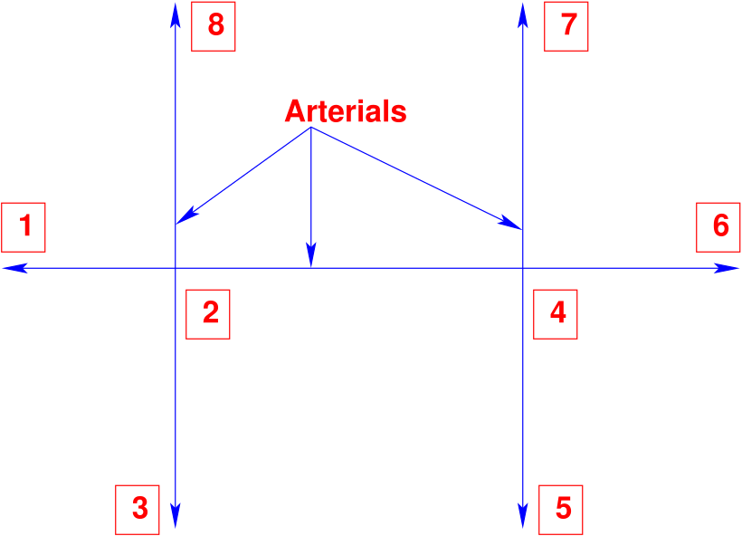
For the given Urban street system geometry and Data inputs determine the performance measurement using Corridor analysis.

Given that:

1. Average vehicle occupancy (AVO) is 1.2.

2. Peak Hour Demand data all Volumes are in (veh/hr) is given in Table. 2.

   control	North bound			South bound			East bound			West bound
   point	Lt	Th	Rt	Lt	Th	Rt	Lt	Th	Rt	Lt	Th	Rt
   2	53	268	34	378	536	176	163	963	55	110	779	110
   4	43	684	109	144	810	153	113	1065	81	126	945	145

3. Capacities, Lengths, Free flow speeds and average flow speeds for each link input data is also given in Table. 3.

   link		length	Capacity	FFS	Actual
   		(km)	(veh/hr)	(km/hr)	speed(km/hr)
   1	2	1.06	1400	56	40
   2	1	1.06	3400	56	56
   2	4	1.67	1400	56	41
   4	2	1.67	1400	56	46
   2	8	1.21	1400	56	43
   8	2	1.21	1700	56	26
   2	3	0.09	3400	56	40
   3	2	0.09	1400	56	12
   4	7	1.21	1400	56	43
   7	4	1.21	1200	56	43
   4	6	0.76	3400	56	56
   6	4	0.76	1400	56	33
   4	5	0.09	3400	56	40
   5	4	0.09	1400	56	11

Solution:

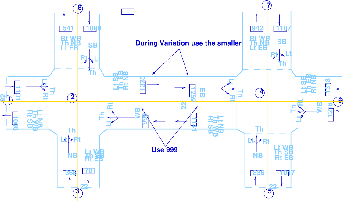
1. Step 1. Because we have Traffic count data we should convert it as link data. This can be done by allocating the flow and adding the volume as per its logical direction (Table 4 col (3)). The flow allocation overview is as shown below. In Fig. 3

   

2. Step 2. Calculate V/C ratio demand by capacity for each link which is as shown below in Table. 5 col (5).
3. Step 3. For V/C \(>\) 1 find the Queued vehicles simply the difference of demand to capacity.
4. Step 4. Adjust the demand downstream till it reaches 10% of the volume before doing further check up. Until all V/C ratios are below 1.

5. Step 5. Determination of person hour delay (PHD), person hours travel (PHT), person kilometer hour travel (PkmT).
   

   link		Demand(V)	Capacity(C)	V/c
   (1)	(2)	(3)	(4)	(5)
   1	2	1181	1400	0.843571
   2	1	1008	3400	0.296471
   2	4	1375	1400	0.899286
   4	2	1141	1400	0.713571
   2	8	541	1400	0.386429
   8	2	1090	1700	0.641176
   2	3	701	3400	0.206176
   3	2	355	1400	0.253571
   4	7	942	1400	0.672857
   7	4	1107	1200	0.9225
   4	6	1318	3400	0.387647
   6	4	1216	1400	0.868571
   4	5	1017	3400	0.299118
   5	4	836	1400	0.597143

   Note that in Table. 5

   1. None of them(V/C) is greater of unity.
   2. No Adjustment is required.
   3. Indicates No Queue delay Determination

   Link		Len.	Dem-	FFS	Actual	free	actual	Free	Actual	Delay
   			and	speed	speed	VHT	VHT	PHT	PHT	PHT	Total
   (1)	(2)	(3)	(4)	(5)	(6)	(7)	(8)	(9)	(10)	(11)	(12)
   1	2	1.06	1181	56	40	22.35	31.30	26.83	37.56	10.73	1251.86
   2	1	1.06	1008	56	56	19.08	19.08	22.90	22.90	0.00	1068.48
   2	4	1.67	1375	56	41	41.00	56.01	49.21	67.21	18.00	2296.25
   4	2	1.67	1141	56	46	34.03	41.42	40.83	49.71	8.88	1905.47
   2	8	1.21	541	56	43	11.69	15.22	14.03	18.27	4.24	654.61
   8	2	1.21	1090	56	26	23.55	50.73	28.26	60.87	32.61	1318.9
   2	3	0.09	701	56	40	1.13	1.58	1.35	1.89	0.54	63.09
   3	2	0.09	355	56	12	0.57	2.66	0.68	3.20	2.51	31.95
   4	7	1.21	942	56	43	20.35	26.51	24.42	31.81	7.38	1139.82
   7	4	1.21	1107	56	43	23.92	31.15	28.70	37.38	8.68	1339.47
   4	6	0.76	1318	56	56	17.89	17.89	21.46	21.46	0.00	1001.68
   6	4	0.76	1216	56	33	16.50	28.00	19.80	33.61	13.80	924.16
   4	5	0.09	1017	56	40	1.63	2.29	1.96	2.75	0.78	91.53
   5	4	0.09	836	56	11	1.34	6.84	1.61	8.21	6.60	75.24
   		12.18	13828				Sum	282.05	396.81	114.76	13162.51

6. Step 6. Free VHT (col(7))= (col (3) \(\times \) col (4))/col (5)
7. Step 7. Actual VHT (col(8))= \(Q_d\) +(col (3) \(\times \) col (4))/col (6), where, \(Q_d\) is the queue delay in our case zero.
8. Step 8. Free PHT (col(9))= AVO \(\times \) col (7)
9. Step 9. Actual PHT (col(10))= AVO \(\times \) col (7)

10. Step 10. Travel Delay (PHD) (col(11))= Actual PHT (col(10)) - Free PHT (col(9))

    Facility type	Length	PkmT	PHT	PHD	Speed(S)
    	(Km)	Pers. Km	Pers. Hr	Pers. Hr	km/hr
    Arterial sub. system	12.8	15795	396.8	114.75	39.6

11. Step 11. Calculation of PkmT

    \begin {eqnarray*} PkmT = AVO \times \Sigma V \times L \end {eqnarray*}

    where, \( V\) is adjusted volume, \(L\) is length of the Link, and \(\Sigma VL\) is col(12) last cell in Table. 5.

12. Step 12. Intensity measures

    \begin {eqnarray*} PHT &=& \Sigma {actual PHT} \\ &=& 396.8 pers.hr \\ t &=& \frac {60 \times PHT}{AVO \times \Sigma V} = 1.43 min/pers \\ S &=& \frac {PkmT}{PHT} = AVO \times ( \Sigma _{d,l,h} [V \times L])/PHT \\ &=& 39.6 km/hr \\ d &=& 3600 \times \frac {(PHT - PHT_f)}{P} \\ & =& 24.9 sec/pers. \end {eqnarray*}

5 Summary

Corridor Analysis is the method of combining Point, Segment and Facility analysis to estimate the overall performance of multi-modal corridor. Mostly the performance measures of any corridor are determined by calculating its capacity, the travel time and queue delay in the given section. Since this tool is required for multi facility and multi-modal transportation system mostly it covers Highway subsystems (Freeways, Rural highways and urban streets) and Transit.

Exercises

1. Not Available

References

1. Urban transportation planning model update - phase ii, 1981. Task F- Development of Corridor Analysis Procedures.
2. Highway Capacity manual part V Draft Working Paper 385-9. University of Florida Transportation Research Center and T-Concepts Corp, Proposed 2010 Highway Capacity manual part V Draft Working Paper 385-9, 2007., 2010.
3. Highway Capacity Manual. Transportation Research Board. National Research Council, Washington, D.C., 2000.

Acknowledgments

I wish to thank several of my students and staff of NPTEL for their contribution in this lecture. I wish to thank specially my student Mr. Ashu Bekelle for his assistance in developing the lecture note, and my staff Ms. Reeba in typesetting the materials. I also appreciate your constructive feedback which may be sent to tvm@civil.iitb.ac.in. Prof. Tom V. Mathew, Department of Civil engineering, Indian Instiute of Technology Bombay, India.