Transport problems are very critical one to be solved frequently, sequentially and economically for all sectors of one nation. Even though these solutions are mandatory, they are continuous and expensive so needs to be planned systematically. These all requirements will lead us to Transportation System Planning. Transportation System Planning is a tool that attempts to provide feasible and systematic method for solving transport problems of the society. Transportation system planning starts from the problem of the society which is the difference of users desire to the existing condition of the system. Afterwards following its stages it will attempt to meet its goals and objectives. While in the process so many analyses are required to be done from them the one is done to know the performance of the existing system. This can be expressed as either individual component performance or the whole system performance. Doing this is dependent on the type of transportation system. Among them multi modal multi facility system is the one which requires aggregate performance measurement for all components which constitutes. According to our study area we can choose from the two methods of performance measurement alternatives which are Corridor analysis and Area wide analysis.
The terminologies used in the corridor analysis is provided below.
Transits are a means of transporting massive either passenger or freight on a separated route. These modes of transportations are a key to every city especially in urban areas. The most common types of Transits include:
Capacity is the maximum hourly flow rate, at which persons or vehicles reasonably can be expected to traverse a point or a uniform section, of a lane or roadway during a given time period, under prevailing roadway, traffic and control conditions. But sometimes the demand may exceed the capacity during peak hours, which will bring queue delay. Thus demand adjustment is required and is done as follows. Adjusting for excess demand from the capacity is necessary only if working with forecasted or estimated demands rather than counted traffic. If the demand exceeds the capacity at any point in time or space, then the excess demand must be stored on the segment and carried over to the following hour. The downstream demands are reduced by the amount of excess demand stored on the segment. The algorithm starts with the entry gate segments on the periphery of the corridor and works inward until all segment demands have been checked against their capacity.
The following steps are used to adjust demand when excess demand occurs in a time period.
 | (1) |
where, i is the current analysis period, i- 1 is the previous analysis period, queuei-1 is the queue remaining from the preceding analysis period.
The segment free-flow traversal times are obtained by dividing the length of the segment by the estimated free-flow speed (FFS), as shown in equation 2
 | (2) |
where, Rf is the Segment free-flow travel time for given Direction of Segment and Time Period, (hr), L is the length of segment (km), and Sf is the Segment free-flow speed computed (km/hr). The FFS is computed according to the Part III methods using the adjusted demands determined in the previous step. The computation is repeated for each direction of each segment for each time sub-periods.
The queuing delay only the amount due to demand exceeding capacity is computed for all segments. The queuing delay is computed for each direction of each segment and time period only when demand is greater than Capacity by eqn. 3.
![Di = T2-× Di-1 +[V - c]× T22-](web2x.png) | (3) |
where, Di is the total delay due to excess demand (veh-hr) for direction, segment, and time period; T is the duration of time sub-period (hr); Di-1 is the queue left over at end of previous time period (veh); V is the demand rate for current time period (veh/hr); and c is the capacity of segment in subject direction (veh/hr). These the above steps are repeated for any additional time periods to be analyzed. For example, if the peak period lasts for 4 hours, it might be divided into four 1hr periods (or 16 quarter hr periods), with each time period analyzed in sequence. The first and the last analysis periods must be uncongested for all delay to be included in the performance measures. Once all time periods have been analyzed, the performance measures are computed.
This step describes how to compute performance measures of congestion intensity, duration, extent, variability, and accessibility for the corridor.
The possible performance measures for the intensity of congestion on the highway subsystems (freeway, two-lane highway, and arterial) in the corridor are computed from one or more of the following: person-hours of travel, person-hours of delay, mean trip speed, and mean trip delay. If average vehicle occupancy (AVO) data are not available, then the performance measures are computed in terms of vehicle-hours rather than person-hours.
![PHT = AV O × Σd,l,h[V × R+ DQ ]](web3x.png) | (4) |
where, PHT is the person-hours of travel in corridor, AV O is the average vehicle occupancy, V is the vehicle demand in Direction on Link during Time Period (veh), R is the segment traversal time (h/km), and DQ is the queuing delay (veh-h).
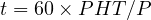 | (5) |
where, t is the mean trip time (min/person), PHT is the person-hours of travel, and P is the total number of person trips.
![S = PkmT--= AV O × Σd,l,h[V-×-L]
P HT P HT](web5x.png) | (6) |
where, S is the mean corridor trip speed (km/h), PkmT is the person-kilometers of travel, PHT is the person-hours of travel, AV O is the average vehicle occupancy, V is the vehicle demand in the given Direction on a Segment and Period (veh), and L is the length of segment (km).
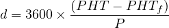 | (7) |
where, d is the mean trip delay (s/person), PHT is the person-hours of travel, PHTf is the person-hours of travel under free-flow conditions, and P is the total number of person trips.
Performance measurements of duration can be computed from the number of hours of congestion observed on any segment. The duration of congestion is the sum of the length of each analysis sub-periods for which the demand exceeds capacity. The duration of congestion (i.e., over-saturation) for any link is computed using Eqn. 8 as:-
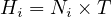 | (8) |
where, Hi is the duration of congestion for Link i(h), Ni is the number of analysis sub-periods for which v∕c > 1.00 on Link i, and T is the duration of analysis sub-periods (h). The maximum duration on any link indicates the amount of time before congestion is completely cleared from the corridor.
Performance measures of the extent of congestion can be computed from the sum of the length of queuing on each segment. One can also identify segments in which the queue overflows the storage capacity; this is particularly useful for ramp metering analyses. To compute the queue length, an assumption must be made about the average density of vehicles in a queue. Default values are suggested in Table. 1
| Sub system | Storage Density | Vehicle Spacing |
| (veh/Km/ln) | (m) | |
| Freeway | 75 | 13.3 |
| Two lane highway | 130 | 7.5 |
| Urban Street | 130 | 7.5 |
To compute queue length, Eqn. 9 is used.
![QL = T-×-[v--c]
N × ds](web8x.png) | (9) |
where, QL is the queue length (km) for the given Direction, of Segment, for Time Sub-period; v is the segment demand (veh/h); c is the segment capacity (veh/h); N is the number of lanes; ds is the storage density (veh/km/ln); and T is the duration of analysis period (h). Note that if v < c, then QL = 0, and if QL > L, then the queue overflows the storage capacity. The queue lengths for all segments then can be added up to obtain the length of queuing in kilometers in the subsystem during the analysis period. The number of segments in which the queue exceeds the storage capacity also might be reported. This statistics is particularly useful for identifying queue overflows that result from ramp metering.
Variability is a sensitivity measure. The variability or sensitivity of the results can be determined by substituting higher and lower demand estimates. For example assuming 110 percent of the original demand estimates for all segments and repeating the calculations.
Accessibility can be measured in terms of the number of trip destinations reachable within a selected travel time for a designated set of origin locations such as a residential zone. The results for each origin zone are tabulated and reported as X percent of the homes in the study area can reach Y percent of the jobs within Z minutes.
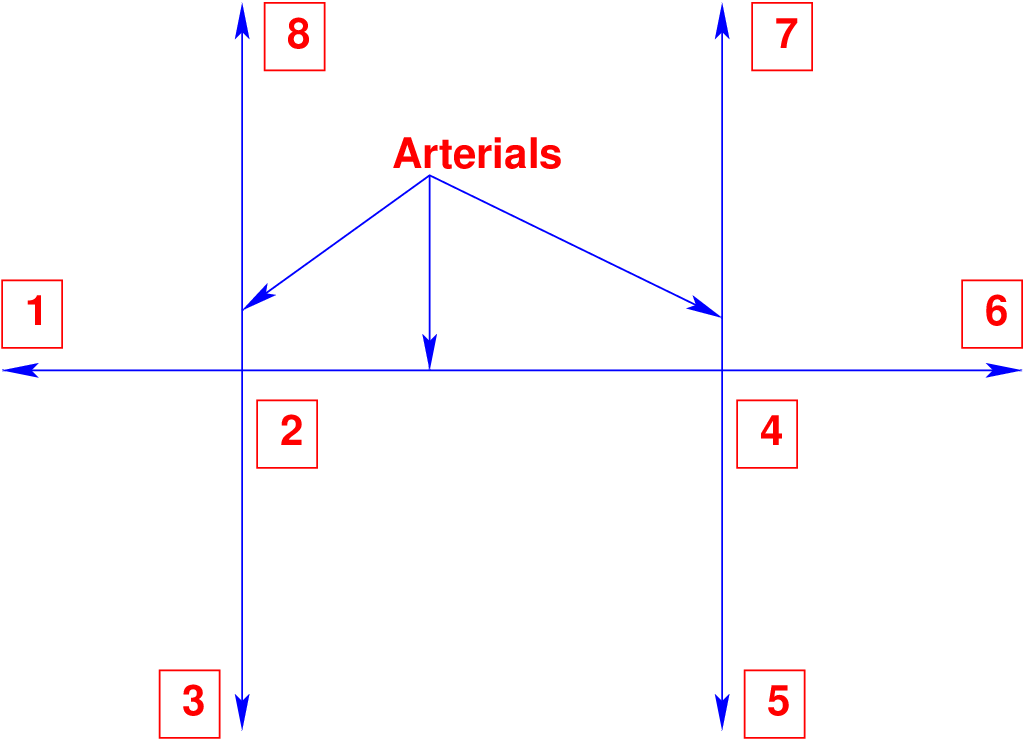
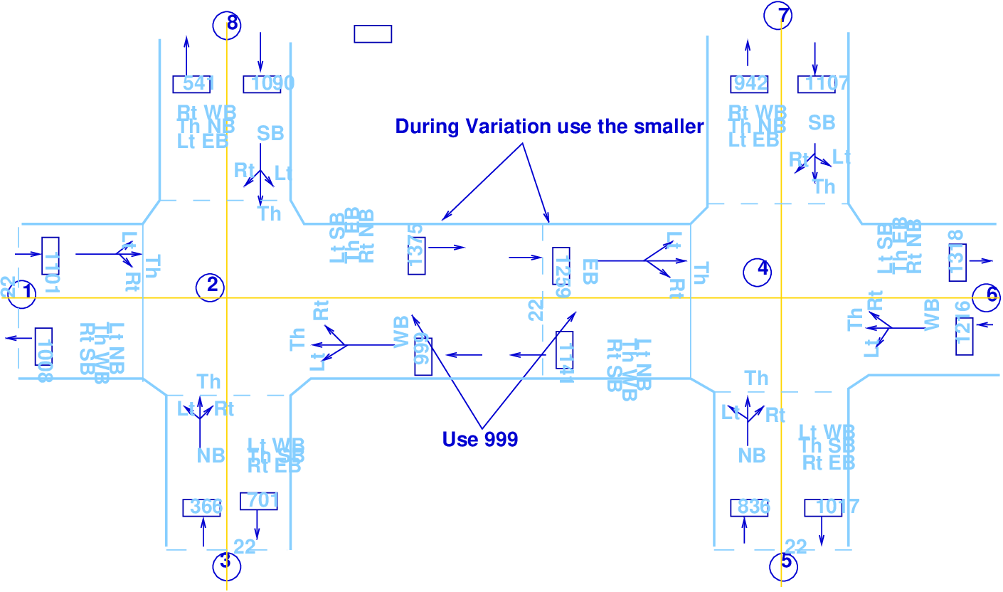
For the given Urban street system geometry and Data inputs determine the performance measurement using Corridor analysis.
Given that:
| control | North bound | South bound | East bound | West bound | ||||||||
| point | Lt | Th | Rt | Lt | Th | Rt | Lt | Th | Rt | Lt | Th | Rt |
| 2 | 53 | 268 | 34 | 378 | 536 | 176 | 163 | 963 | 55 | 110 | 779 | 110 |
| 4 | 43 | 684 | 109 | 144 | 810 | 153 | 113 | 1065 | 81 | 126 | 945 | 145 |
link | length | Capacity | FFS | Actual | |
| (km) | (veh/hr) | (km/hr) | speed(km/hr) | ||
| 1 | 2 | 1.06 | 1400 | 56 | 40 |
| 2 | 1 | 1.06 | 3400 | 56 | 56 |
| 2 | 4 | 1.67 | 1400 | 56 | 41 |
| 4 | 2 | 1.67 | 1400 | 56 | 46 |
| 2 | 8 | 1.21 | 1400 | 56 | 43 |
| 8 | 2 | 1.21 | 1700 | 56 | 26 |
| 2 | 3 | 0.09 | 3400 | 56 | 40 |
| 3 | 2 | 0.09 | 1400 | 56 | 12 |
| 4 | 7 | 1.21 | 1400 | 56 | 43 |
| 7 | 4 | 1.21 | 1200 | 56 | 43 |
| 4 | 6 | 0.76 | 3400 | 56 | 56 |
| 6 | 4 | 0.76 | 1400 | 56 | 33 |
| 4 | 5 | 0.09 | 3400 | 56 | 40 |
| 5 | 4 | 0.09 | 1400 | 56 | 11 |
| link | Demand(V) | Capacity(C) | V/c | |
| (1) | (2) | (3) | (4) | (5) |
| 1 | 2 | 1181 | 1400 | 0.843571 |
| 2 | 1 | 1008 | 3400 | 0.296471 |
| 2 | 4 | 1375 | 1400 | 0.899286 |
| 4 | 2 | 1141 | 1400 | 0.713571 |
| 2 | 8 | 541 | 1400 | 0.386429 |
| 8 | 2 | 1090 | 1700 | 0.641176 |
| 2 | 3 | 701 | 3400 | 0.206176 |
| 3 | 2 | 355 | 1400 | 0.253571 |
| 4 | 7 | 942 | 1400 | 0.672857 |
| 7 | 4 | 1107 | 1200 | 0.9225 |
| 4 | 6 | 1318 | 3400 | 0.387647 |
| 6 | 4 | 1216 | 1400 | 0.868571 |
| 4 | 5 | 1017 | 3400 | 0.299118 |
| 5 | 4 | 836 | 1400 | 0.597143 |
Note that in Table. 5
| Link | Len. | Dem- | FFS | Actual | free | actual | Free | Actual | Delay
| ||
| and | speed | speed | VHT | VHT | PHT | PHT | PHT | Total | |||
| (1) | (2) | (3) | (4) | (5) | (6) | (7) | (8) | (9) | (10) | (11) | (12) |
| 1 | 2 | 1.06 | 1181 | 56 | 40 | 22.35 | 31.30 | 26.83 | 37.56 | 10.73 | 1251.86 |
| 2 | 1 | 1.06 | 1008 | 56 | 56 | 19.08 | 19.08 | 22.90 | 22.90 | 0.00 | 1068.48 |
| 2 | 4 | 1.67 | 1375 | 56 | 41 | 41.00 | 56.01 | 49.21 | 67.21 | 18.00 | 2296.25 |
| 4 | 2 | 1.67 | 1141 | 56 | 46 | 34.03 | 41.42 | 40.83 | 49.71 | 8.88 | 1905.47 |
| 2 | 8 | 1.21 | 541 | 56 | 43 | 11.69 | 15.22 | 14.03 | 18.27 | 4.24 | 654.61 |
| 8 | 2 | 1.21 | 1090 | 56 | 26 | 23.55 | 50.73 | 28.26 | 60.87 | 32.61 | 1318.9 |
| 2 | 3 | 0.09 | 701 | 56 | 40 | 1.13 | 1.58 | 1.35 | 1.89 | 0.54 | 63.09 |
| 3 | 2 | 0.09 | 355 | 56 | 12 | 0.57 | 2.66 | 0.68 | 3.20 | 2.51 | 31.95 |
| 4 | 7 | 1.21 | 942 | 56 | 43 | 20.35 | 26.51 | 24.42 | 31.81 | 7.38 | 1139.82 |
| 7 | 4 | 1.21 | 1107 | 56 | 43 | 23.92 | 31.15 | 28.70 | 37.38 | 8.68 | 1339.47 |
| 4 | 6 | 0.76 | 1318 | 56 | 56 | 17.89 | 17.89 | 21.46 | 21.46 | 0.00 | 1001.68 |
| 6 | 4 | 0.76 | 1216 | 56 | 33 | 16.50 | 28.00 | 19.80 | 33.61 | 13.80 | 924.16 |
| 4 | 5 | 0.09 | 1017 | 56 | 40 | 1.63 | 2.29 | 1.96 | 2.75 | 0.78 | 91.53 |
| 5 | 4 | 0.09 | 836 | 56 | 11 | 1.34 | 6.84 | 1.61 | 8.21 | 6.60 | 75.24 |
| 12.18 | 13828 | Sum | 282.05 | 396.81 | 114.76 | 13162.51 | |||||
| Facility type | Length | PkmT | PHT | PHD | Speed(S) |
| (Km) | Pers. Km | Pers. Hr | Pers. Hr | km/hr | |
| Arterial sub. system | 12.8 | 15795 | 396.8 | 114.75 | 39.6 |

![P HT == Σ3a9c6t.u8aplerPsH.Thr
60× P HT
t = AV-O-×-ΣV- = 1.43min ∕pers
P kmT
S = ------ = AV O × (Σd,l,h[V × L ])∕PHT
PHT
= 39.6km∕hr
d = 3600× (P-HT---P-HTf-)
P
= 24.9sec∕pers.](web10x.png)
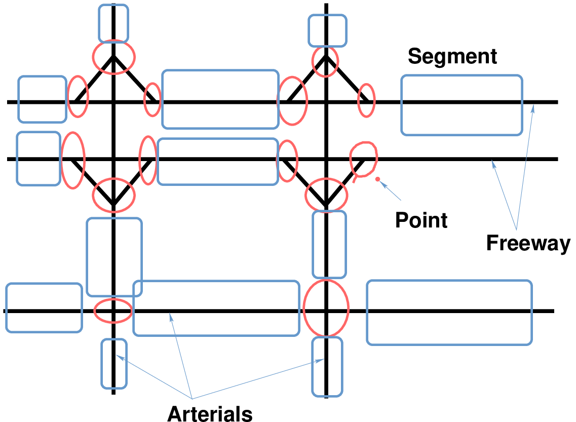
Corridor Analysis is the method of combining Point, Segment and Facility analysis to estimate the overall performance of multi-modal corridor. Mostly the performance measures of any corridor are determined by calculating its capacity, the travel time and queue delay in the given section. Since this tool is required for multi facility and multi-modal transportation system mostly it covers Highway subsystems (Freeways, Rural highways and urban streets) and Transit.
I wish to thank several of my students and staff of NPTEL for their contribution in this lecture. I wish to thank specially my student Mr. Ashu Bekelle for his assistance in developing the lecture note, and my staff Ms. Reeba in typesetting the materials. I also appreciate your constructive feedback which may be sent to tvm@civil.iitb.ac.in
Prof. Tom V. Mathew
Department of Civil Engineering
Indian Institute of Technology Bombay, India
_________________________________________________________________________
Wednesday 27 September 2023 10:44:57 PM IST