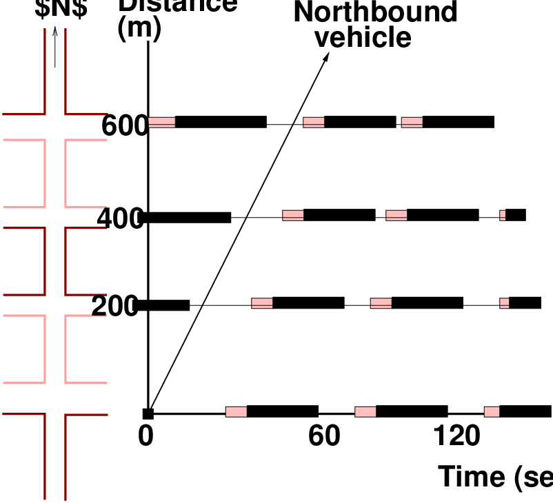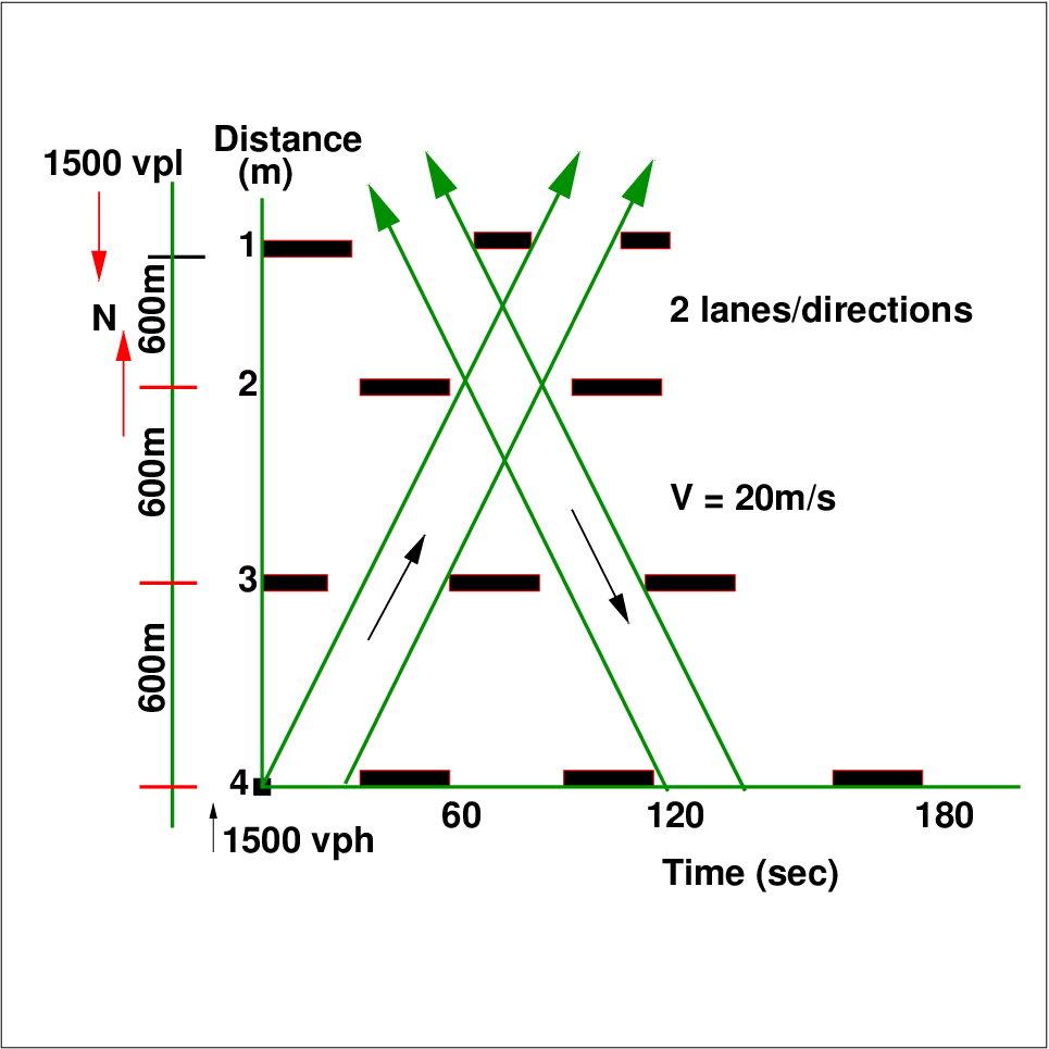
Figure 1: Vehicle trajectory
This chapter covers basic aspects of traffic signal coordination. Signal coordination is done when they are closely space to enable vehicle in one predominant direction to get continuous green. This will reduce the delay and travel time in one direction and increases throughput. The design principles of signal coordination will be presented in this chapter.
For signals that are closely spaced, it is necessary to coordinate the green time so that vehicles may move efficiently through the set of signals. In some cases, two signals are so closely spaced that they should be considered to be one signal. In other cases, the signals are so far apart that they may be considered independently. Vehicles released from a signal often maintain their grouping for well over 335m.
There are four major areas of consideration for signal coordination:
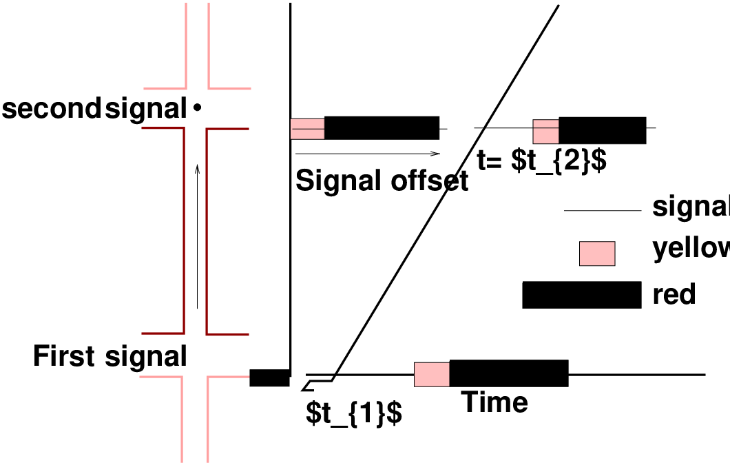
The most complex signal plans require that all signals have the same cycle length. Fig. 1 illustrates path (trajectory) that a vehicle takes as time passes. At t = t1, the first signal turns green. After some lag, the vehicle starts and moves down the street. It reaches the second signal at some time t = t2. Depending on the indication of that signal, it either continues or stops. The difference between the two green initiation times is referred to as the signal offset, or simply as the offset. In general, the offset is defined as the difference between green initiation times, measured in terms of the downstream green initiation relative to the upstream green initiation.
It is common to consider the benefit of a coordination plan in terms of a cost or penalty function; a weighted combination of stops and delay, and other terms as given here:
 | (1) |
The object is to make this dis-benefit as small as possible. The weights A and B are coefficients to be specified by the engineer or analyst. The values of A and B may be selected so as to reflect the estimated economic cost of each stop and delay. The amounts by which various timing plans reduce the cost, can then be used in a cost-benefit analysis to evaluate alternative plans. The conservation of energy and the preservation of the environment have grown in importance over the years. Given that the vehicles must travel, fuel conservation and minimum air pollution are achieved by keeping vehicles moving as smoothly as possible at efficient speeds. This can be achieved by a good signal-coordination timing plan. Other benefits of signal coordination include, maintenance of a preferred speed, possibility of sending vehicles through successive intersections in moving platoons and avoiding stoppage of large number of vehicles.
The physical layout of the street system and the major traffic flows determine the purpose of the signal system. It is necessary to consider the type of system, whether one-way arterial, two-way arterial, one-way,two-way, or mixed network. the capacities in both directions on some streets, the movements to be progressed, determination of preferential paths
Among the factors limiting benefits of signal coordination are the following:
All signals cannot be easily coordinated. When an intersection creating problems lies directly in the way of the plan that has to be designed for signal coordination, then two separate systems, one on each side of this troublesome intersection, can be considered. A critical intersection is one that cannot handle the volumes delivered to it at any cycle length.
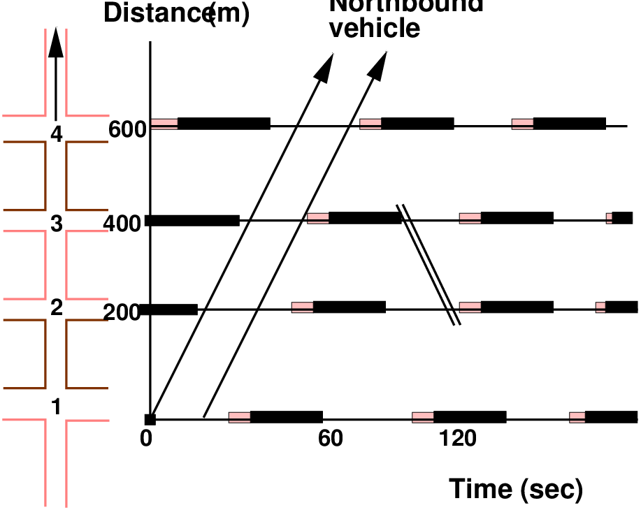
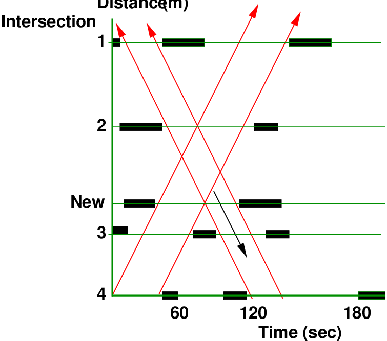
The time-space diagram is simply the plot of signal indications as a function of time for two or more signals. The diagram is scaled with respect to distance, so that one may easily plot vehicle positions as a position of time. Fig. 2 is a time-space diagram for two intersections.
The standard conventions are used in Fig. 2: a green signal indication is shown by a blank or thin line, amber by a shaded line and red by a solid line. For purpose of illustration of trajectory in the time space diagram for intersections, a northbound vehicle going at a constant speed of 40fps is shown. The ideal offset is defined as the offset that will cause the specified objective to be best satisfied. For the objective of minimum delay, it is the offset that will cause minimum delay. In Fig. 2, the ideal offset is 25 sec for that case and that objective. If it is assumed that the platoon was moving as it went through the upstream intersection then the ideal offset is given by
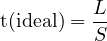 | (2) |
where: t(ideal) = ideal offset,sec, L = block length, m, S = vehicle speed, mps.
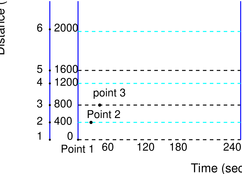
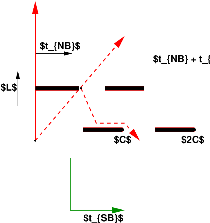
In Fig. 3 a one-way arterial is shown with the link lengths indicated. Assuming no vehicles are queued at the signals, the ideal offsets can be determined if the platoon speed is known. For the purpose of illustration, a platoon speed of 60 fps is assumed. The offsets are determined according to Eqn. 2. Next the time-space diagram is constructed according to the following rules:
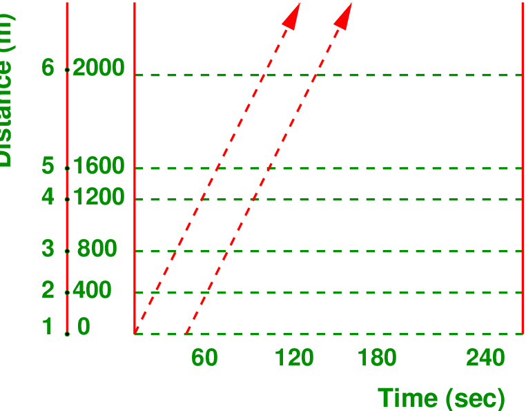
Fig. 4 shows the time-space diagram for the illustration mentioned previously. Fig. 5 explores some features of the time-space diagram.
It sometimes happens that there are vehicles stored in block waiting for a green light. These may be stragglers from the last platoon, vehicles that turned into the block, or vehicles that came out of parking lots or spots. The ideal offset must be adjusted to allow for these vehicles, so as to avoid unnecessary stops. The ideal offset can then be given as:
 | (3) |
where, Q = number of vehicles queued per lane, veh, h= discharge headway of queued vehicle, sec/veh, and Loss1 = loss time associated with vehicles starting from rest at the first downstream signal.
If it is known that there exists a queue and its size is known approximately, then the link offset can be set better than by pretending that no queue exists. There can be great cycle-to-cycle variation in the actual queue size, although its average size may be estimated. Even then, queue estimation is a difficult and expensive task and should be viewed with caution.
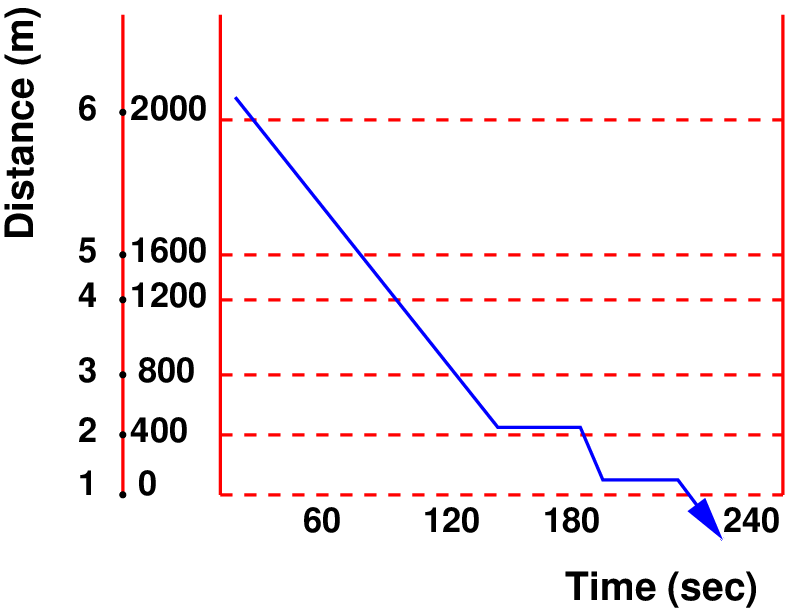
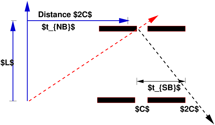
Consider that the arterial shown in Fig. 3 is not a one-way but rather a two-way street.
Fig. 6 shows the trajectory of a southbound vehicle on this arterial.
If any offset were changed in Fig. 6 to accommodate the southbound vehicle(s), then the northbound vehicle or platoon would suffer. The fact that offsets are interrelated presents one of the most fundamental problems of signal optimization. The inspection of a typical cycle (as in Fig. 7) yields the conclusion that the offsets in two directions add to one cycle length. For longer lengths (as in Fig. 8) the offsets might add to two cycle lengths. When queue clearances are taken into account, the offsets might add to zero lengths.
The general expression for the two offsets in a link on a two-way street can be written as
 | (4) |
where the offsets are actual offsets, n is an integer and C is the cycle length. Any actual offset can be expressed as the desired ideal offset, plus an error or discrepancy term:
 | (5) |
where j represents the direction and i represents the link.
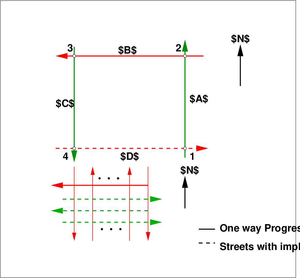
A one-way street system has a number of advantages, not the least of which is traffic elimination of left turns against opposing traffic. The total elimination of constraints imposed by the closure of loops within the network or grid is not possible. Fig. 9 highlights the fact that if the cycle length, splits, and three offsets are specified, the offset in the fourth link is determined and cannot be independently specified. Fig. 9 extends this to a grid of one-way streets, in which all of the north-south streets are independently specified. The specification of one east-west street then locks in all other east-west offsets. The key feature is that an open tree of one-way links can be completely independently set, and that it is the closing or closure of the open tree which presents constraints on some links.
The bandwidth concept is very popular in traffic engineering practice, because
The efficiency of a bandwidth (measured in seconds) is defined as the ratio of the bandwidth to the cycle length, expressed as a percentage:
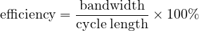 | (6) |
An efficiency of 40% to 50% is considered good. The bandwidth is limited by the minimum green in the direction of interest.
Fig. 10 illustrates the bandwidths for one signal-timing plan. The northbound efficiency can be estimated as (17∕60)100% = 28.4%. There is no bandwidth through the south-bound. The system is badly in need of re-timing at least on the basis of the bandwidth objective. In terms of vehicles that can be put through this system without stopping, note that the northbound bandwidth can carry 17∕2.0 = 8.5 vehicles per lane per cycle in a nonstop path through the defined system. The northbound direction can handle
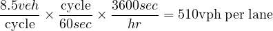
 | (7) |
where: BW = measured or computed bandwidth, sec, L= number of through lanes in indicated direction, h = headway in moving platoon, sec/veh,and C =cycle length.
The engineer usually wishes to design for maximum bandwidth in one direction, subject to some relation between the bandwidths in the two directions. There are both trial-and-error and somewhat elaborate manual techniques for establishing maximum bandwidths. Refer to Fig. 11, which shows four signals and decent progressions in both the directions. For purpose of illustration, assume it is given that a signal with 50:50 split may be located midway between Intersections 2 and 3. The possible effect as it appears in Fig. 12 is that there is no way to include this signal without destroying one or the other through band, or cutting both in half. The offsets must be moved around until a more satisfactory timing plan develops. A change in cycle length may even be required. The changes in offset may be explored by:
There is no need to produce new strips for each cycle length considered: all times can be made relative to an arbitrary cycle length ‘C. The only change necessary is to change the slope(s) of the guidelines representing the vehicle speeds. The northbound vehicle takes 3600∕60 = 60sec to travel from intersection 4 to intersection 2. If the cycle length C = 120sec, the vehicle would have arrived at intersection 2 at C∕2, or one half of the cycle length. To obtain a good solution through trial-and-error attempt, the following should be kept in consideration:
An elegant mathematical formulation requiring two hours of computation on a supercomputer is some-what irrelevant in most engineering offices. The determination of good progressions on an arterial must be viewed in this context:only 25 years ago, hand held calculators did not exist; 20 years ago, calculators had only the most basic functions. 15 years ago, personal computers were at best a new concept. Previously, engineers used slide rules. Optimization of progressions could not depend on mathematical formulations simply because even one set of computations could take days with t he tools available. Accordingly,graphical methods were developed. The first optimization programs that took queues and other details into account began to appear, leading to later developments that produced the signal-optimization programs in common use in late 1980s. As computers became more accessible and less expensive, the move to computer solutions accelerated in the 1970s. New work on the maximum-bandwidth solution followed with greater computational power encouraging the new formulations.
Simple progression is the name given to the progression in which all the signals are set so that a vehicle released from the first intersection will arrive at the downstream intersections just as the signals at those intersections initiate green. As the simple progression results in a green wave that advances with the vehicles, it is often called a forward progression. It may happen that the simple progression is revised two or more times in a day, so as to conform to the direction of the major flow, or to the flow level. In this case, the scheme may be referred to as a flexible progression. Under certain circumstances, the internal queues are sufficiently large that the ideal offset is negative. The downstream signal must turn green before the upstream signal, to allow sufficient time for the queue to start moving before the arrival of the platoon. The visual image of such a pattern is of the green marching upstream, toward the drivers in the platoon. This is referred to as reverse progression.
In certain geometries it is possible to obtain very effective progressions in both directions on two-way streets. The existence of these patterns presents the facts that:
The traffic engineer may well be faced with a situation that looks intimidating, but for which the community seek to have smooth flow of traffic along an arterial or in a system. The orderly approach begins with first, appreciating the magnitude of the problem. The splits, offsets, and cycle length might be totally out of date for the existing traffic demand. Even if the plan is not out of date, the settings in the field might be totally out of date, the settings in the field might be totally different than those originally intended and/or set. Thus, a logical first step is simply to ride the system and inspect it. Second, it would be very useful to sketch out how much of the system can be thought of as an open tree of one way links. A distinction should be made among
Downtown grids might well fall into the last category, at least in some cases. Third, attention should focus on the combination of cycle length, block length and platoon speed and their interaction. Fourth, if the geometry is not suitable, one can adapt and fix up the situation to a certain extent. Another issue to address, of course, is whether the objective of progressed movement of traffic should be maintained.
The problem of oversaturation is not just one of degree but of kind - extreme congestion is marked by a new phenomenon: intersection blockage. The overall approach can be stated in a logical set of steps:
Signalization can be improved through measures like, reasonably short cycle lengths, proper offsets and proper splits. Sometimes when there is too much traffic then options such as equity offsets(to aid cross flows) and different splits may be called upon. A metering plan involving the three types - internal, external and release - may be applied. Internal metering refers to the use of control strategies within a congested network so as to influence the distribution of vehicles arriving at or departing from a critical location. External metering refers to the control of the major access points to the defined system, so that inflow rates into the system are limited if the system if the system is already too congested. Release metering refers to the cases in which vehicles are stored in such locations as parking garages and lots, from which their release can be in principle controlled.
The concept of signal coordination is presented in this chapter. Coordination in one way is simple and effective and results in better progression. Two-way coordination is complex and less effective. Bandwidth is an important parameter in evaluating the efficiency of coordination. Further, the concepts of forward and reverse progression are introduced.
I wish to thank several of my students and staff of NPTEL for their contribution in this lecture. I also appreciate your constructive feedback which may be sent to tvm@civil.iitb.ac.in
Prof. Tom V. Mathew
Department of Civil Engineering
Indian Institute of Technology Bombay, India
_________________________________________________________________________
Thursday 28 September 2023 10:47:34 AM IST