This chapter is an attempt to provide a basic knowledge about the fuel consumption and vehicular emissions. The concepts of air pollution and automobile pollution are also given due importance. Various types of numerical models related to fuel consumption and air pollution are discussed briefly. The report aims to identify the necessity of understanding the impact of vehicular pollution on the environment. In order to bring the fuel consumption and emission levels to a minimum, various mitigation measures are to be implemented, which are also pointed out in the report.
Urbanization has paved the way for higher levels of comfort and standard of living. Rapid urbanization has thus caused an increase in the number of vehicles and this, on the other hand, is causing another set of problems including lack of space, reduction in natural resources, environmental pollution, etc. We need to consider the existence of a future generation and plan the utilization of our environment and resources wisely. The following sections discuss how the transportation engineering is helpful in bringing about welcome changes in the development of a sustainable environment. For this, we need to have a basic knowledge about fuel consumption, emission and resulting air pollution, which are discussed briefly below.
Fuel efficiency or Fuel Economy is the energy efficiency of a vehicle, expressed as the ratio of distance traveled per unit of fuel consumed in km/liter. Fuel efficiency depends on many parameters of a vehicle, including its engine parameters, aerodynamic drag, weight, and rolling resistance. Higher the value of fuel efficiency, the more economical a vehicle is (i.e., the more distance it can travel with a certain volume of fuel). Fuel efficiency also affects the emissions from the vehicles.
Fuel consumption is the reciprocal of Fuel Efficiency. Hence, it may be defined as the amount of fuel used per unit distance, expressed in liters/100km. Lower is the value of fuel consumption, more economical is the vehicle. That is less amount of fuel will be used to travel a certain distance.
Air Pollution maybe defined as
The disruption caused to the natural atmospheric environment by the introduction of certain chemical substances, gases or particulate matter, which cause discomfort and harm to structures and living organisms including plants, animals and humans.
Air pollution has become a major concern in most of the countries of the world. It is responsible for causing respiratory diseases, cancers and serious other ailments. Besides the health effects, air pollution also contributes to high economic losses. Poor ambient air quality is a major concern, mostly in urban areas. Air pollution is also responsible for serious phenomena such as acid rain and global warming.
The substances causing air pollution are collectively known as air pollutants. They may be solid, liquid or gaseous in nature. Pollutants are classified as primary and secondary air pollutants. Primary pollutants are those which are emitted directly to atmosphere, whereas, secondary pollutants are formed through chemical reactions and various combinations of the primary pollutants. Some of the major primary and secondary air pollutants are given in Table. 1 and Table. 2.
| Sulphur Oxides (SOx) | Carbon Monoxide (CO) |
| Nitrogen Oxides (NOx) | Carbon Dioxide (CO2) |
| Volatile Organic Compounds (V OC) | Hydrocarbons (HC) |
| Ammonia (NH3) | Particulate Matter (PM) |
| Radioactive pollutants | Chlorofluorocarbons (CFC) |
| Toxic Metals like Lead, Cadmium and Copper
| |
| Photochemical smog |
| Peroxyacetyl Nitrate (PAN) |
| Ozone (O3) |
The sources of air pollution may be natural or anthropogenic. The anthropogenic sources of air pollution are those which are caused by human activity. The major anthropogenic sources include Stationary sources (such as smoke stacks of power plants, incinerators, and furnaces), Mobile sources (e.g. motor vehicles, aircraft), Agriculture and industry (e.g. chemicals, dust), Fumes from paint, hair spray, aerosol sprays, Waste deposits in landfills (which contain methane) and Military (e.g. Nuclear weapons, toxic gases). The natural sources of air pollution may be Dust from areas of low vegetation, Radon gas from radioactive decay of Earth’s crust, Smoke and CO from wildfires, and volcanic activity which produces sulfur, chlorine and particulates.
The pollution caused due to the emissions from vehicles is generally referred to as automobile pollution. The transportation sector is the major contributor to air pollution. Vehicular emissions are of particular concerns, since these are ground level sources and hence have the maximum impact on the general population. The rapid increase in urban population have resulted in unplanned urban development, increase in consumption patterns and higher demands for transport and energy sources, which all lead to automobile pollution. The automobile pollution will be higher in congested urban areas. The vehicle obtains its power by burning the fuel. The automobile pollution is majorly caused due to this combustion, which form the exhaust emissions, as well as, due to the evaporation of the fuel itself. The chemical reactions occurring during ideal combustion stages may be represented as follows:
|
| (1) |
Similarly, the typical engine combustion which occurs in vehicles can be represented by the below chemical equation.
 | (2) |
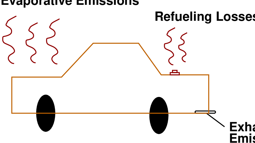
The fuel loss of vehicles may be due to emissions or refuelling. The emissions maybe evaporative or exhaust emissions. The fuel losses in a vehicle are shown in Fig. 1.
The pollutants which are emitted from the exhaust pipe of the automobiles are known as exhaust pollutants. They are formed as a result of combustion of the fuel in the engine. These pollutants are harmful to the atmosphere and living things in particular. The major types of exhaust pollutants are discussed in the following sections.
Combustion of petroleum generates Sulfur Dioxide. It is a colorless, pungent and non – flammable gas. It causes respiratory illness, but occurs only in very low concentrations in exhaust gases. Further oxidation of SOx forms H2SO4 and thus acid rains.
Combustion under high temperature and pressure emits Nitrogen dioxide. It is reddish brown gas. Nitrogen oxides contribute to the formation of ground level Ozone and acid rain.
Hydrocarbons result from the incomplete combustion of fuels. Their subsequent reaction with the sunlight causes smog and ground level Ozone formation. V OCs are a special group of Hydrocarbons. They are divided into 2 types – methane and non – methane. Prolonged exposure to some of these compounds (like Benzene, Toluene and Xylene) may also cause Leukemia.
It is an indicator of complete combustion of the fuel. Although it does not directly affect our health, it is a greenhouse gas which causes global warming.
It is a product of the incomplete burning of fuel and is formed when Carbon is partially oxidized. CO is an odorless, colorless gas, but is toxic in nature. It reaches the blood stream to form Carboxyhemoglobin, which reduces the flow of Oxygen in blood.
It is a malleable heavy metal. Lead present in the fuel helps in preventing engine knock. Lead causes harm to the nervous and reproductive systems. It is a neurotoxin which accumulates in the soft tissues and bones.
These are tiny solid or liquid particles suspended in gas (soot or smoke). Particulate Matter in higher concentrations may lead to heart diseases and lung cancer.
The vehicular emissions are due to a variety of factors. The emissions vary according to the environment, fuel quality, vehicle, etc. emissions are higher in congested and urban areas. Fuel adulteration and overloading also cause higher amount of emissions. The emissions from vehicles depend on the following factors:
The number of trips, distance travelled and driving mode are the major travel related factors affecting emissions. As the number of trips increases, the amounts of emissions also increase. Emissions increase with the distance travelled by the vehicle. The vehicular emissions also depend on the driving mode. The driving modes may be idling, cruising, acceleration and deceleration. These modes complete one driving cycle. Other factors affecting the emission rates are the speed, acceleration and engine load of the vehicle. Low speeds, congested driving conditions, sharp acceleration, deceleration, etc. result in higher emissions. On the other hand, intermediate speeds and low density traffic conditions cause lower emissions.
These include the geometric design features of the highway such as grade. The emission rate is very high at steep gradients, as the vehicle needs to put in more effort to maintain its speed. The highway network facilities such as signalized intersections, freeway ramps, toll booths, weaving sections, etc. also influence the vehicular emission rates.
Vehicle related factors include the engine sizes, horsepower and weight of the vehicle. Vehicles with large engine sizes emit more pollutants. Since larger sized engines are seen in vehicles with more horsepower and more weight, these factors also contribute to the emission rates. Another important factor is the age of the vehicle. Older vehicles have higher emission rates.
Bharat Stage emissions standards are emissions standards instituted by the Government of the Republic of India that regulate the output of certain major air pollutants (such as nitrogen oxides (NOx), carbon monoxide (CO), hydrocarbons (HC), particulate matter (PM), sulfur oxides (SOx)) by vehicles and other equipment using internal combustion engines. They are comparable to the European emissions standards. India started adopting European emission and fuel regulations for four-wheeled light-duty and for heavy-dc from the year 2000. For two and three wheeled vehicles, the Indian emission regulations are applied. As per the current requirement, all transport vehicles must carry a fitness certificate which is to be renewed each year after the first two years of new vehicle registration. The National Fuel Policy announced on October 6, 2003, a phased program for implementing the EU emission standards in India by 2010. The implementation schedule of EU emission standards in India is summarized in Table. 3.
| Standard | Reference | Date | Region |
| India 2000 | Euro 1 | 2000 | Nationwide |
| 2001 | NCR*, Mumbai, Kolkata, Chennai | ||
| Bharat Stage II | Euro 2 | 2003.04 | NCR*, 13 Cities** |
| 2005.04 | Nationwide | ||
| Bharat Stage III | Euro 3 | 2005.04 | NCR*, 13 Cities** |
| 2010.04 | Nationwide | ||
| Bharat Stage IV | Euro 4 | 2010.04 | NCR*, 13 Cities** |
Some of the important emission standards for different vehicle types are given in the following tables (Table. 4 - 7).
| Year | Reference | Test | CO | HC | NOx | PM |
| 1992 | - | ECE | 17.3- | 2.7-3.7 | - | - |
| R49 | 32.6 | |||||
| 1996 | - | ECE | 11.2 | 2.4 | 14.4 | - |
| R49 | ||||||
| 2000 | Euro I | ECE | 4.5 | 1.1 | 8 | 0.36* |
| R49 | ||||||
| 2005** | Euro II | ECE | 4 | 1.1 | 7 | 0.15 |
| R49 | ||||||
| 2010** | Euro III | ESC | 2.1 | 0.66 | 5 | 0.1 |
| ETC | 5.45 | 0.78 | 5 | 0.16 | ||
| 2010# | Euro IV | ESC | 1.5 | 0.46 | 3.5 | 0.02 |
| ETC | 4 | 0.55 | 3.5 | 0.03 | ||
| Year | CO | HC | HC + NOx |
| 1991 | Dec- | 08- | - |
| 30 | Dec | ||
| 1996 | 6.75 | - | 5.4 |
| 2000 | 4 | - | 2 |
| 2005 (BS II) | 2.25 | - | 2 |
| 2010.04 (BS III) | 1.25 | - | 1.25 |
| Year | CO | HC | HC + NOx |
| 1991 | Dec- | 08- | - |
| 30 | Dec | ||
| 1996 | 5.5 | - | 3.6 |
| 2000 | 2 | - | 2 |
| 2005 (BS II) | 1.5 | - | 1.5 |
| 2010.04 (BS III) | 1 | - | 1 |
| Year | Reference | CO | HC | HC + NOx | NOx |
| 1991 | - | 14.3- | 2.0- | - | |
| 27.1 | 2.9 | ||||
| 1996 | - | 8.68- | - | ||
| 12.4 | 3.00-4.36 | ||||
| 1998* | - | 4.34- | - | ||
| 6.20 | 1.50-2.18 | ||||
| 2000 | Euro 1 | 2.72- | - | ||
| 6.90 | 0.97-1.70 | ||||
| 2005** | Euro 2 | 2.2-5.0 | - | 0.5-0.7 | |
| 2.3 | 0.2 | 0.15 | |||
| 2010** | Euro 3 | 4.17 | 0.25 | - | 0.18 |
| 5.22 | 0.29 | 0.21 | |||
| 1 | 0.1 | 0.08 | |||
| 2010# | Euro 4 | 1.81 | 0.13 | - | 0.1 |
| 2.27 | 0.16 | 0.11 | |||
Fuel consumption models are mathematical functions relating the various factors contributing to the fuel consumption. The influencing factors may be no. of vehicle trips, distance travelled by the vehicle, no. of stops, vehicle’s average speed, etc. The major fuel consumption models are discussed in the following sections.
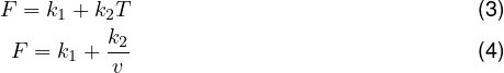
Average speed models are macroscopic in nature. They are concerned with the traffic network as a whole, on a large scale. Individual vehicles are not considered. This model relates the fuel consumption directly with the travel time (or indirectly with vehicle speeds). This model is not valid for speeds higher than 56 km/hr. as the effects of air resistance become increasingly stronger. The fuel consumed is related to the average speed (or travel time) using the relation below:
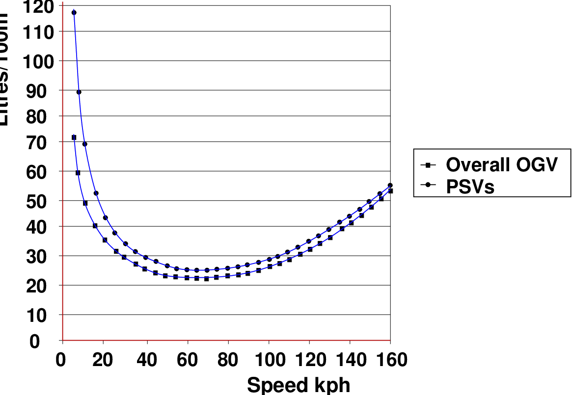
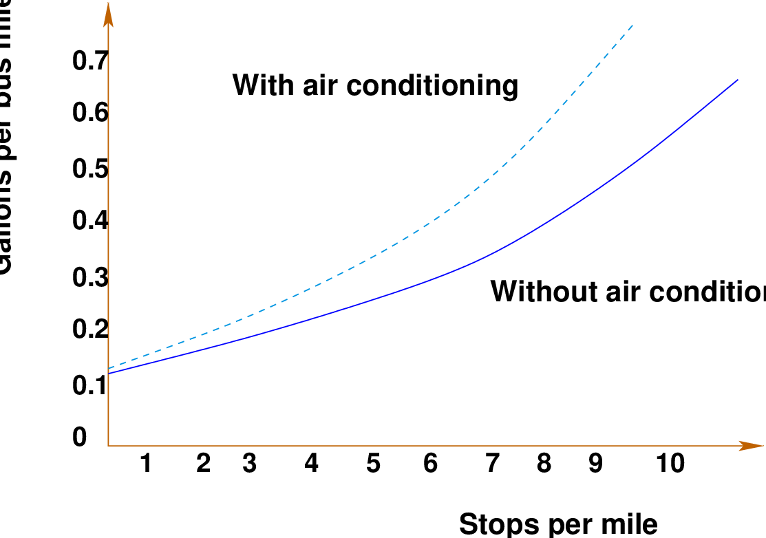
where, F = Fuel consumed per vehicle per unit distance (liters/km), T = Travel time per unit distance, including stops and speed changes (minutes/km), v = Avg. speed measured over a distance including stops and speed changes (10 ≤ v ≤ 56kmph), k1 = parameter associated with fuel consumed to overcome rolling resistance, approximately proportional to vehicle weight (liters/veh- km), k2 = Parameter approximately proportional to fuel consumption while idling (liters/hr).Fig. 2 gives the relation between fuel and consumption and speed of the vehicle. It can be inferred from the figure that fuel consumption is high for lower speeds and is the minimum for intermediate speeds.Fig. 3 shows the relation between bus fuel consumption and number of stops. It is clear from the graph that fuel consumption increases as the number of stops of the vehicle increases.
A city has a total of 20000 commuters travelling at an average speed of 25kmph, and using an arterial road of length 15 km. Due to the congestion and parking problems, 35% commuters form car pools with a car occupancy of 3.0 and 20% arrange for subscription bus service (50 seater). Rest of the commuters choose to travel by private cars. The peak period congestion was found to be reduced and the speed was increased to 35kmph. Assuming the no. of stops to be 7, calculate the amount of fuel saved. Take k1 = 0.085liters/km, k2 = 1.5 liters/hr.
Solution: It is required to find the difference in fuel consumption between the two cases. In the first case, all commuters use private cars (i.e. car occupancy 1) and in the second case, some of them use public transport services, while others still use private cars.
In the first case, there were a total of 20000 commuters with car occupancy = 1, speed 25kmph and the distance to be travelled is 15 km. from the equation 3, we have: Total fuel consumption, F = k1 + k2∕v. Thus for the distance of 15km travelled, the total fuel consumption is equal to [0.085 * 15] + [(1.5/25) * 15], which is 2.175 liters/vehicle. Thus for a total of 20000 commuters, the fuel consumption will be 2.175 * 20000 which is equal to 43500 liters.
In the second case, the vehicles move with a new speed of 35kmph, and out of the total 20000 commuters, 35% (0.35 * 20000 = 7000) form car pools with occupancy 3.0. Hence, the number of car pool vehicles is 7000/3, that is 2333 vehicles. 20% (0.20 * 20000 = 4000) of the commuters use a 50 seater bus service. Hence the number of buses will be 4000/50, which is equal to 80 buses. Remaining (20000 - 7000 - 4000 = 9000) are single car drivers. The total consumption by car will include the consumption of cars of single occupancy and the cars in the car pool. Hence, the fuel consumption by cars is [0.085 * 15] + [(1.5/35) * 15], that is 1.917 liters/vehicles. So, for all the cars, the total fuel consumption will be 1.917* (9000 + 2333), which is 21725.36 liters. Similarly, the bus fuel consumption for a bus with 7 stops will be 0.3 *2.35 * 80 * 15 which is 846 liters.
Fuel consumption corresponding to 7 stops is obtained from Fig. 3. 2.35 is a conversion factor to bring the fuel consumption in terms of liters/km instead of gallons/mile. Total fuel consumption will be the sum of fuel consumptions of bus and car. That is 21725+846 = 22571 liters. The total amount of fuel saved will be the difference of fuel consumptions in both the cases. Hence the amount of fuel saved is 43500 - 2257, which is equal to 20929 liters.
Unlike the average speed model, the drive model elemental model is a microscopic fuel consumption model. It considers the movement of a single vehicle. This model is used to obtain the fuel consumption rates during various vehicle operating conditions or drive mode. The different drive modes include cruising, idling, accelerating and decelerating, which together form a driving cycle. The important assumptions used in this model are that the driving mode elements are independent of each other and the sum of the component consumption equals the total amount of fuel consumed. The advantages of this model are that the model is simple and general and there is a direct relationship to existing traffic modelling techniques. The disadvantage of this model is that the variation in the behavior of different drivers and behavior of the same driver under different situations is ignored.The component elements considered here are various drive modes such as cruising, idling and accelerating. The total fuel consumed for the drive mode elemental model is given by the relation:
 | (5) |
where, G = fuel consumed per vehicle over a measured distance (total section distance), L = total section distance traveled, D = stopped delay per vehicle (time spent in idling), S = number of stops, f1 = fuel consumption rate per unit distance while cruising, f2 = fuel consumption rate per unit time while idling, f3 = excess fuel used in decelerating to stop and accelerating back to cruise speed
The total fuel consumption by a vehicle travelling on a stretch of road is 0.0735 liters/veh-km. The average stopped delay for the vehicle is 6s. The vehicle stops thrice during its journey. Assume f1 = 0.0045, f2 = 0.0035 and f3 = 0.002. Calculate the length of road considered. If the vehicle is cruising throughout the stretch of the road, what is the decrease in fuel consumption?
Solution: From the equation. 5, the fuel consumed per vehicle over a measured distance is given by

Step 1: It is given that fuel consumed per vehicle is 0.0735 liters/veh-km, average delay is 6s and the number of stops are 3. The values of f1, f2 and f3 are given as 0.0045,0.0035 and 0.002 respectively. It is required to find the length of the road. The length L can be computed from the above equation as given: 0.0735 = (0.0045 *L) + (0.0035 * 6) + (0.002 * 3). Therefore, Length, L is equal to 10 km.
Step 2: When the vehicle is cruising throughout the length, there will not be any delays or stops. Therefore, total fuel consumption: G′ = f1L = 0.0045 * 10 = 0.045liters∕veh - km.
Step 3: The decrease in fuel consumption is will be the difference in fuel consumptions as obtained in steps 1 and 2, which is 0.0735-0.045 = 0.0285 liters/veh-km.
Instantaneous fuel consumption models are derived from a relationship between the fuel consumption rates and the instantaneous vehicle power. Second-by-second vehicle characteristics, traffic conditions and road conditions are required in order to estimate the expected fuel consumption. Due to the disaggregate characteristic of fuel consumption data, these models are usually implemented to evaluate individual transportation projects such as single intersections, toll plazas, sections of highway, etc. In this model the fuel consumption rate is taken as the function of different variables such as weight of vehicle, drag coefficient, rolling resistance, frontal area, acceleration and speed, transmission efficiency and grade.
Air Pollution Models give a causal relationship between emissions, meteorology, atmospheric concentrations, deposition, and other factors. They explain the consequences of past and future scenarios and the determination of the effectiveness of abatement strategies. They are also used to describe the concentration of various pollutants in the air. The major types of air pollution models are emission models and dispersion models.
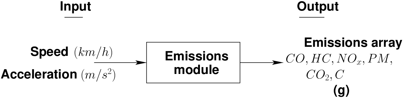
Emission models are commonly used to provide traffic emission information for the prediction and management of air pollution levels near roadways. The model helps in comparing the actual pollution levels with the emission standards set. Hence, the abatement of pollution can also be carried out. The basic schematic diagram of an emission model is given in the Fig. 4.
Emission models estimate the emission quantity using the emission factor. The emission factor may be defined as the ratio of average amount of pollutant discharged to the total amount of the fuel discharged. It is expressed in kg of particulate / metric ton of fuel. The emission factors used in the emission models reflect different levels of congestion. The various types of emission models are briefly discussed in the following paragraphs.
The model is similar to the instantaneous fuel consumption model. It describes the vehicle emission behavior during any instant of time. The advantages of the model are that the emission factors can be calculated and generated for any vehicle operating profile, and the model considers dynamics in driving patterns. The model has some disadvantages also such as: Detailed and precise information on vehicle operation and location is required and The process of data collection is expensive.
This model is useful in macro level where detailed information is not required. A single emission factor is used to represent a particular type of vehicle and general type of driving. Emission is estimated using the equation:
 | (6) |
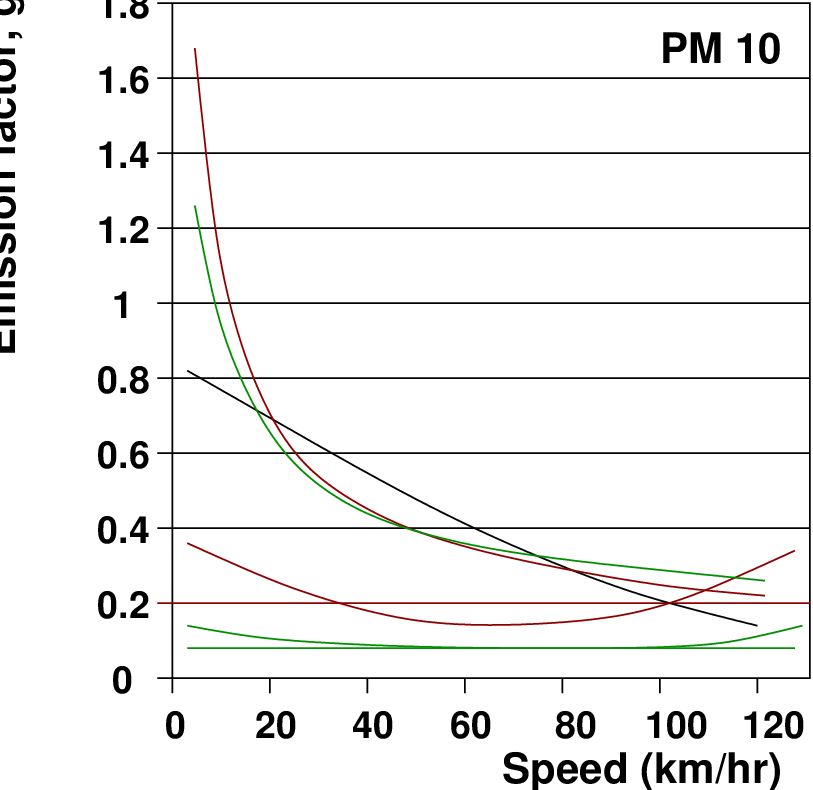
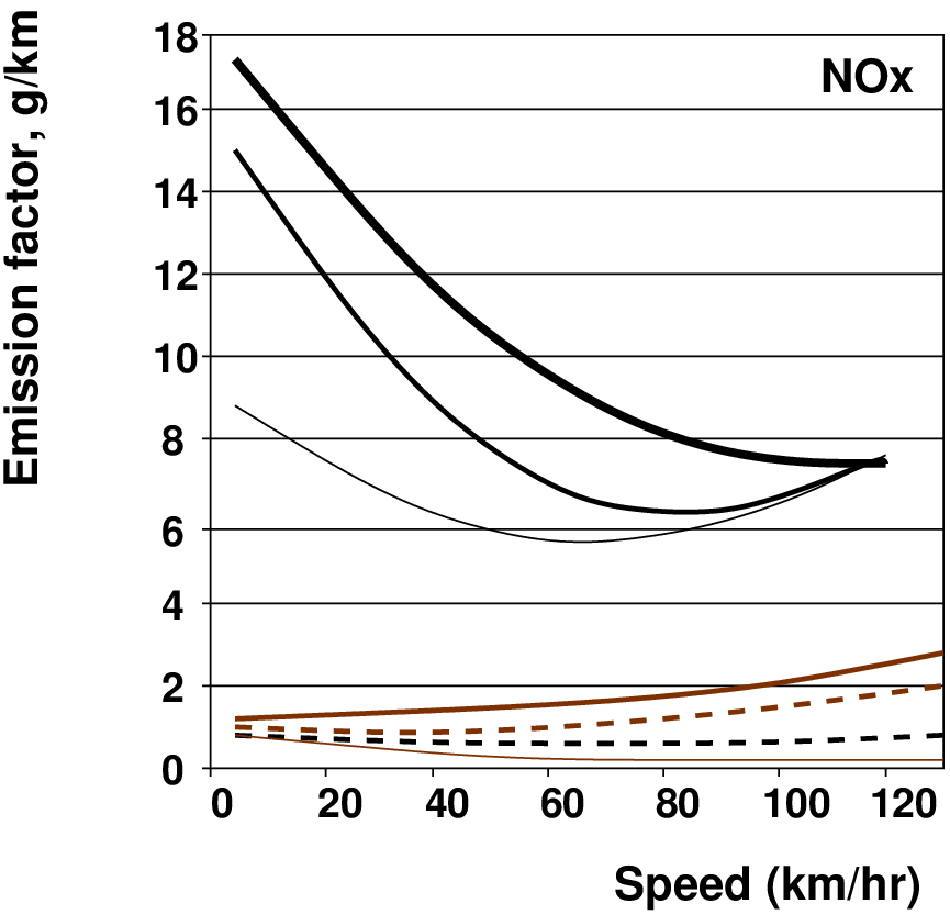
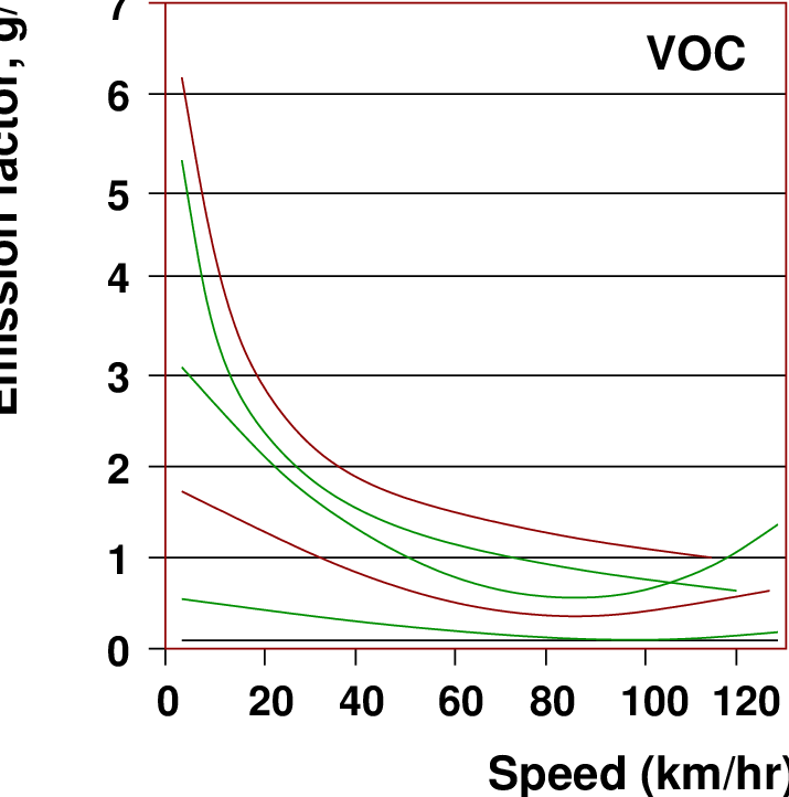
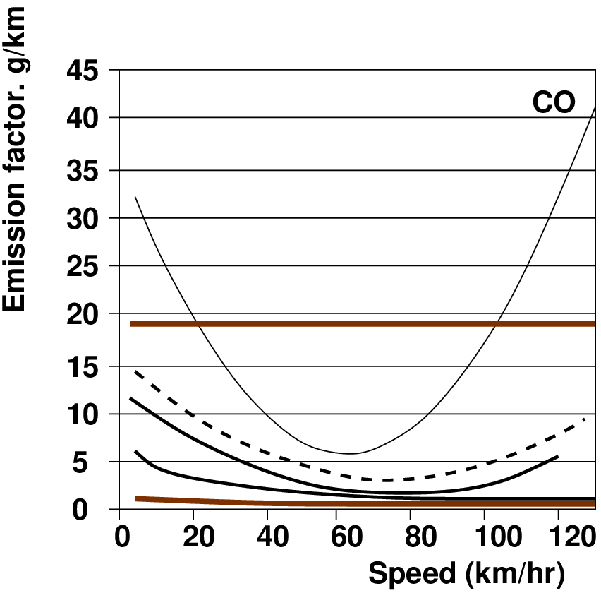
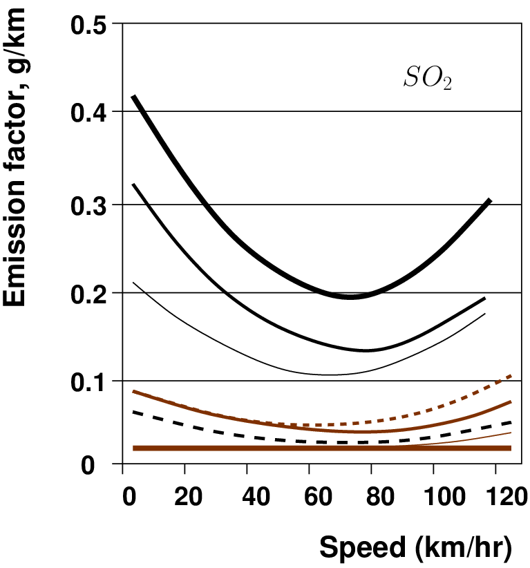
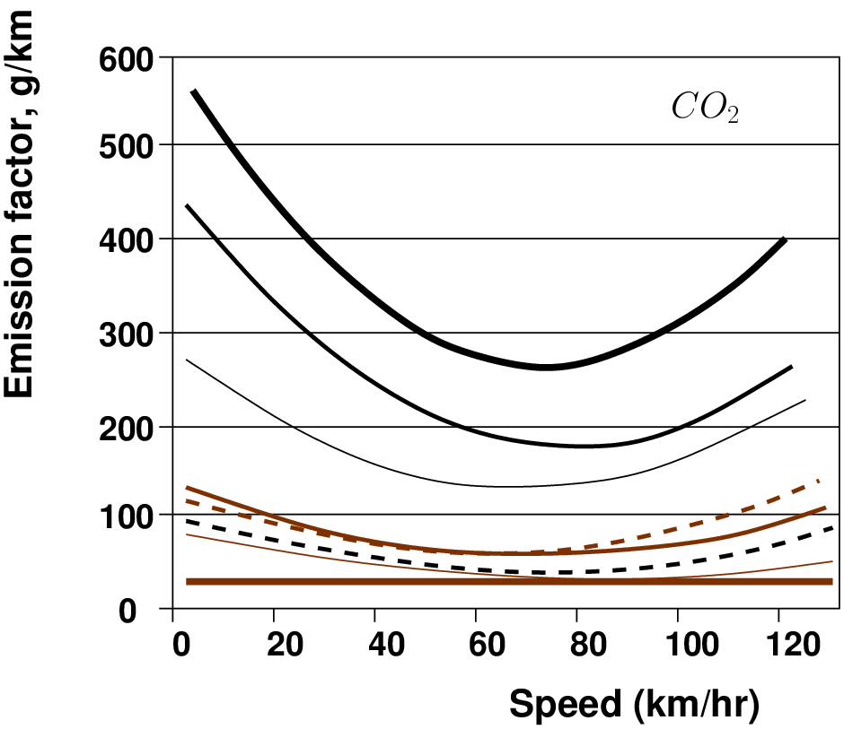
where, E = emissions, in units of pollutant per unit of time, A = activity rate, in units of weight, volume, distance or duration per unit of time, EF = emission factor, in units of pollutant per unit of weight, volume, distance or duration The variation of exhaust emission factors with speed for the major exhaust pollutants are given in the following figures (Fig. 5 to Fig. 10).
For Particulate Matter (PM10) and Volatile Organic Compounds, the emissions steadily decrease with the speed. In case of Nitrogen Oxides, Sulphur Oxides and Carbon Dioxide, the emission is highest for low speeds, decreases for intermediate speeds and then again increases with the speed. For Carbon Monoxide, the highest emission levels occur for higher speeds and minimum emission occurs for intermediate speeds.
Using the emission factor model, the amount of CO emitted by a vehicle was estimated as 50 grams per hour. If the vehicle travelled at a velocity of 40kmph, estimate the emission factor for CO for the vehicle.
Solution It is given that the total emission E is 50g/hr. The activity ‘A’ here is the amount of CO emitted by the vehicle, which is 40km/hr. from the eqn. 6, we have, the total emissions is E = A*EF. Therefore, the emission factor will be E∕A = 50/40 = 1.25. That is, the emission factor of CO is 1.25 grams/km.
Average Speed Models are used in the measurement of emission rates of a pollutant for a given vehicle for various speeds during a trip. Average Speed Emission models, along with the Emission factor models are widely applied in national and regional inventories. The emission factor in this model (EF) is measured over a range of driving cycle (which includes driving, stops, starts, acceleration and deceleration). It is given in g/veh-km. Though these models are good in measuring congestion, they have certain disadvantages, which are explained below:
This model is similar to the drive mode elemental fuel consumption model. Emission rates are explained as a function of the vehicle operation mode. The model provides accurate emission estimates at micro level. For each mode, emission rate is fixed for a particular type of vehicle and pollutant. Instantaneous traffic related data is required to estimate the fuel consumption. The total emission for a trip on a section of road is given by the product of modal emission rate and the time spent in the mode.
Various emission models are available to estimate the contribution of motor vehicle transportation to air pollution. The major vehicular emission models in use are discussed briefly below:
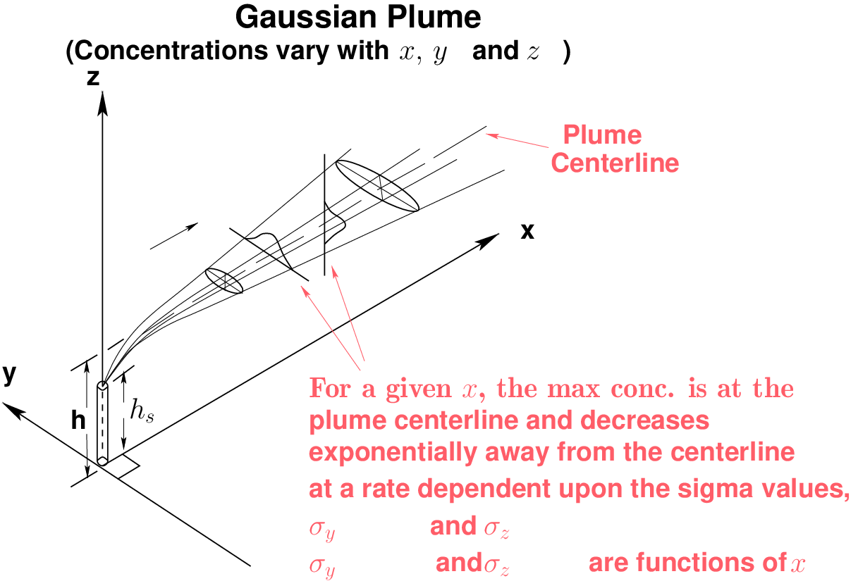
This is a simple mathematical model used to estimate the concentration of pollutants at a point at some distance from the source of emission. This model is used for static as well as mobile sources of emissions. In this model, the dispersion in the three dimensions is calculated. Dispersion in the downwind direction is a function of the mean wind speed blowing across the plume. Air pollution is represented by an idealized plume coming from the top of a stack of some height and diameter. The major assumption in this model is that over short periods of time (such as a few hours), steady state conditions exists with regard to air pollutant emissions and meteorological changes. The prominent limitation of this model is that it is not suitable for pollutants which undergo chemical transformations in the atmosphere. Also, it depends largely on steady state meteorological conditions and is short term in nature.
The Fig. 11 shows the dispersion of pollutants in a Gaussian plume.
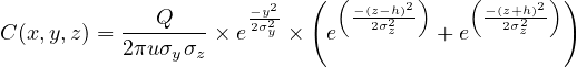
Dispersion in the cross-wind direction and in the vertical direction will be governed by the Gaussian plume equations of lateral dispersion. Lateral dispersion depends on a value known as the atmospheric condition, which is a measure of the relative stability of the surrounding air. The model assumes that dispersion in these two dimensions will take the form of a normal Gaussian curve, with the maximum concentration in the center of the plume. The model maybe used to calculate the Effective Stack Height, Lateral and Vertical Dispersion Coefficients and Ground-Level Concentrations. The Gaussian plume is used to find out the concentration of pollutants at any point in space, and is given by:
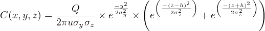 | (7) |
where, C = concentration of the emission (micro grams/cubic meter) at any point x meters downwind of the source, y meters laterally from the centerline of the plume, and z meters above ground level.Q = quantity or mass of the emission (in grams) per unit of time (seconds), u = wind speed (in meters per second), h = height of the source above ground level (in meters), σy and σz are the standard deviations of a statistically normal plume in the lateral and vertical dimensions, respectively. They are functions of x.
A bus stalled at a signal emits pollutants at the rate of 20000g/s. The exhaust pipe is situated at height of 0.75 m from the Ground level. What will be the concentration of pollutants inhaled by a man living on the first floor of a building with storey height 3.5 m? The building is situated at a lateral distance of 5m from the main road and longitudinal distance of 4m downwind of the source. Assume a wind velocity of 10 m/s, σy = 375m and σz = 120m.
Solution: The concentration of the emission is given by eqn. 4.2 which is

Mitigation measures are measures taken to control, reduce or prevent pollution due to automobile emissions. Some of the measures that may be adopted to reduce fuel consumption and air pollution are given below.
Automobiles are large contributer to the environmental pollution. The different fuel consumption and air pollution models discussed in this report help us to estimate how much fuel we are using and the amount of pollutants we are releasing in the atmosphere. As the population and number of vehicles are increasing abruptly, more amounts of pollutants are being discharged. If this trend continues, there will not be any more energy sources left for the future generations. Also, the world will be so polluted that living organisms may not be able to thrive. Hence, we need to understand the importance of saving the environment. Alternate sources of fuels for e.g. renewable sources can be used which also help in reducing the pollution. Our aim must be to preserve the nature and have the environment, along with a sustainable transportation system.
I wish to thank several of my students and staff of NPTEL for their contribution in this lecture. Specially, I wish to thank my student Ms. Soumya Nair for her assistance in developing the lecture note, and my staff Ms. Reeba in typesetting the materials. I also appreciate your constructive feedback which may be sent to tvm@civil.iitb.ac.in
Prof. Tom V. Mathew
Department of Civil Engineering
Indian Institute of Technology Bombay, India
_________________________________________________________________________
Thursday 28 September 2023 11:39:43 AM IST